Explore our entire Camera Modeling Series:

• Part I: Focal Length And Collinearity

• Part 2: Introducing Lens Distortion

• Part 3: Exploring Distortion and Distortion Models

• Part 4: Pinhole Obsession

• Part 5: The Deceptively Asymmetric Unit Sphere

If you’d like to be notified of when that next post drops, just follow us on LinkedIn or subscribe to our newsletter.

—

Previously, we covered some of the basics of camera modeling, and examined the pinhole projection model of a camera. There, we looked at some of the historical context behind how affinity in the image plane has been traditionally modeled, and why different models are preferable.

Today, we want to explore another part of the camera modeling process: modeling lens distortions. One assumption behind our pinhole-projection model is that light travels in straight rays, and does not bend. Of course, our camera's lens is not a perfect pinhole and light rays will bend and distort due to the lens' shape, or due to refraction.

What does lens distortion look like?

Before we get into the actual models themselves, it is good to first understand what lens distortion looks like. There are several distinct types of distortions that can occur due to the lens or imaging setup, each with unique profiles. In total, these are typically broken into the following categories:

1. Symmetric Radial Distortion

2. Asymmetric Radial Distortion

3. Tangential or De-centering Distortion

Each of these is explored independently below. For each of these distortions, consider the base-case where there is no distortion:

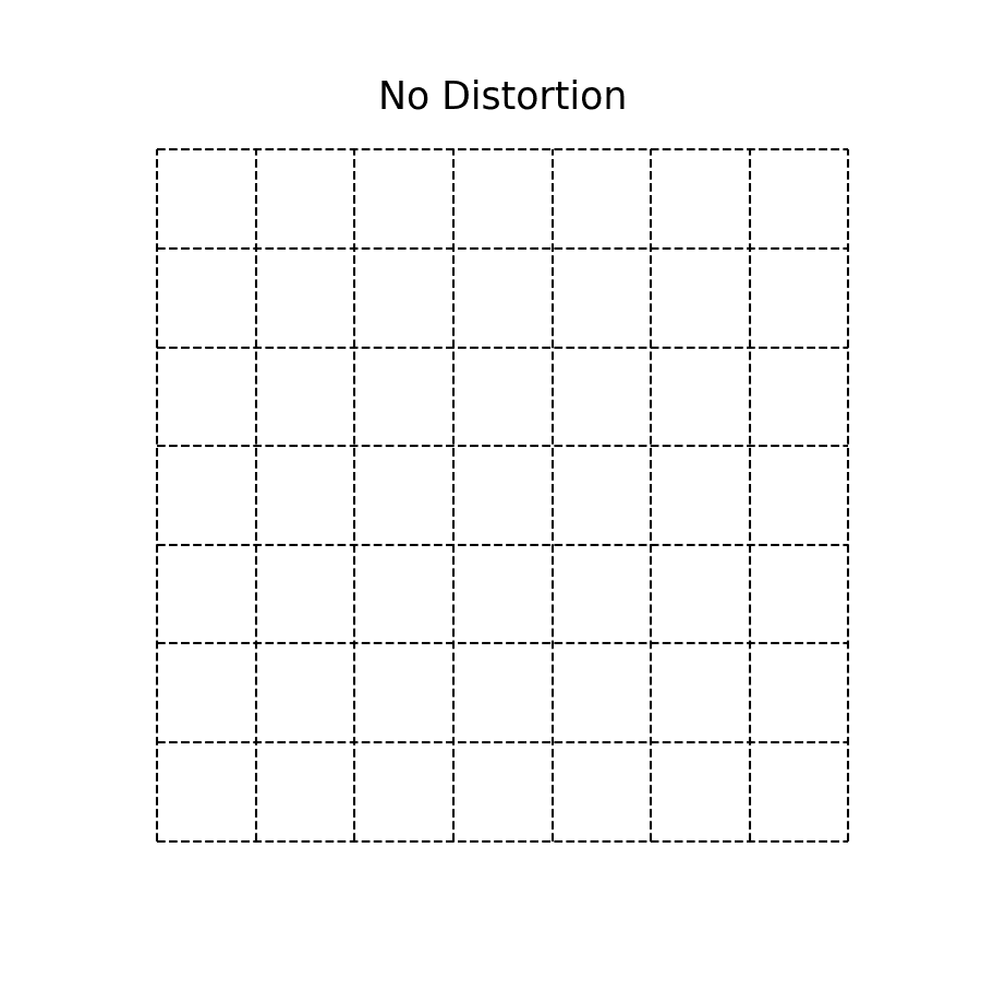
In the above figure, we represent the image plane as a grid. As we discuss the different kinds of distortions, we'll demonstrate how this grid is warped and transformed. Likewise, for any point $(x, y)$ that we refer to throughout this text, we're referring to the coordinate frame of the image plane, centered (with origin) at the principal point. This makes the math somewhat easier to read, and doesn't require us to worry about column and row offsets $c_x$ and $c_y$ when trying to understand the math.

Symmetric Radial Distortions

Symmetric radial distortions are what are typically imagined when discussing image distortion. Often, this type of distortion will be characterized depending on if it is positive (pincushion) or negative (barrel) distortion. Pincushion is "positive" because the projected distance increases beyond the expected locations as one moves farther away from the center of the image plane; likewise, Barrel distortion is "negative" since projected distance goes towards the center.

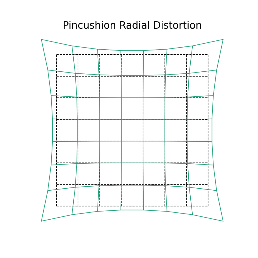
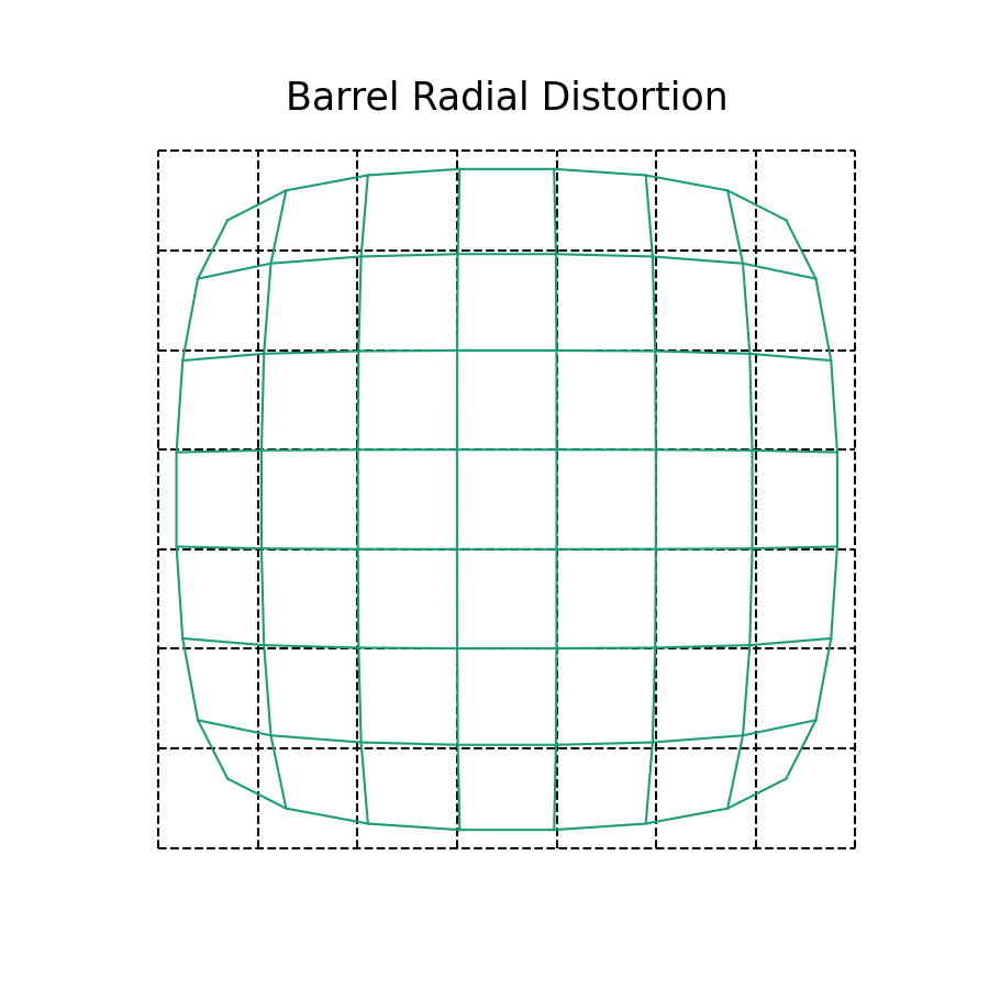
While the two distortions might seem as if they are fundamentally different, they are in fact quite alike! The amount of distortion in the teal lines is greater in magnitude at the edges of our image plane, while being smaller in the middle. This is why the black and teal lines overlap near the center, but soon diverge as distance increases.

Symmetric radial distortion is an after-effect of our lens not being a perfect pinhole. As light enters the lens outside of the perspective center it bends towards the image plane. It might be easiest to think of symmetric radial distortion as if we were mapping the image plane to the convexity or concavity of the lens itself. In a perfect pinhole camera, there wouldn't be any distortion, because all light would pass through a single point!

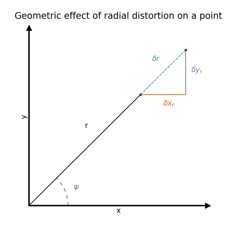
This distortion is characterized as symmetric because it only models distortion as a function of distance from the center of the image plane. The geometric effect of radial distortion is only in the radial direction, as characterized by $\delta r$ in the above figure.

Asymmetric Radial Distortions

Asymmetric radial distortions are radial distortion effects much like the above, but unlike symmetric radial distortion, asymmetric radial distortion characterizes distortion effects that are dependent both on the distance from the image center as well as how far away the object being imaged is. Asymmetric radial effects are most pronounced in two scenarios:

1. Cameras with long focal lengths and very-short relative object distances. e.g. a very-near-field telephoto lens that is capturing many objects very close.

2. Observing objects through a medium of high-refraction, or differing refractive indices. e.g. two objects underwater where one is near and one is far away.

This type of distortion is typically tricky to visualize, as well as to quantify, because it is dependent on the environment. In most robotic and automated vehicle contexts, asymmetric radial distortion is not a great concern! Why? Well, the difference in distortions depends on the difference in distances between objects. This is usually because of some kind of refractive difference between two objects being imaged, or because the objects are out of focus of the camera (i.e. focal length is too large relative to the object distance).

Neither of the above two scenarios are typical; as such, asymmetric radial distortion is an important aspect of modeling the calibration in applications when these scenarios are encountered.

In most robotic contexts, the primary use for imaging and visual odometry is done in relatively short ranges with cameras that have short focal lengths, and the primary medium for light to travel through is air. Since there doesn't tend to be big atmospheric variances between objects that are close, and since light is all traveling through the same medium, there isn't much of an asymmetric refractive effect to characterize or measure. As a result, this kind of radial distortion isn't common when calibrating cameras for these kinds of applications. If we can't measure it, we shouldn't try to model it!

You may be left wondering what is meant by "close" when discussing "atmospheric variance between objects that are close." In short: it is all relative to the refractive index of the medium in which you are imaging. On the ground it is atypical to have atmospheric effects (we don't see pockets of ozone on the ground, as an example).

This is not generally true underwater, nor if you are performing some kind of aerial observation from the stratosphere or higher. Additionally, even in such scenarios, if all observed objects are roughly the same distance away then it doesn't matter since asymmetric radial distortion characterizes radial effects as a result of the extra distance light travels (and refracts) between two objects at different distances from the camera.

Tangential (De-centering) Distortions

The last kind of distortions to characterize in a calibration are tangential effects, often as a result of de-centered lens assemblies. Notice that unlike radial distortion, the image plane is skewed, and the distance from center is less important. The effect is exaggerated; most cameras do not have tangential distortions to this degree.

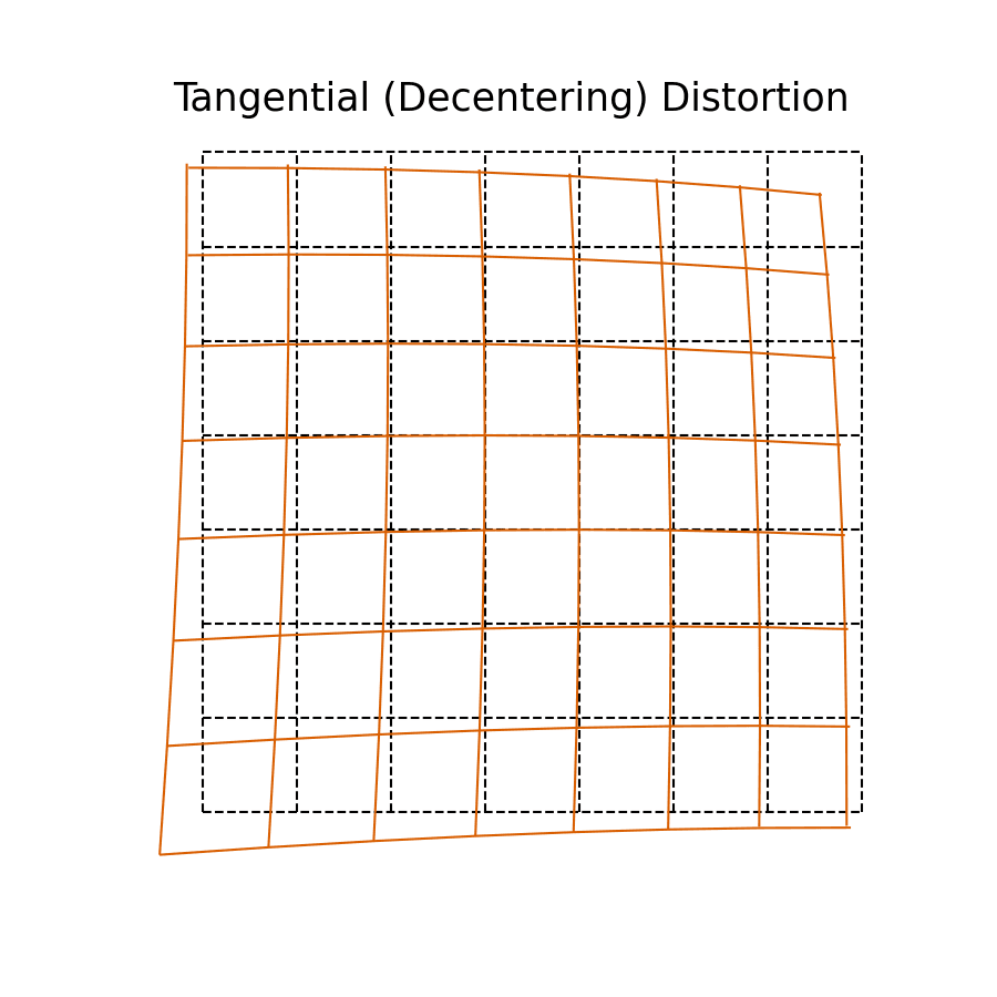
Tangential distortion is sometimes also called de-centering distortion, because the primary cause is due to the lens assembly not being centered over and parallel to the image plane. The geometric effect from tangential distortion is not purely along the radial axis. Instead, as can be seen in the figure above, it can perform a rotation and skew of the image plane that depends on the radius from the image center!

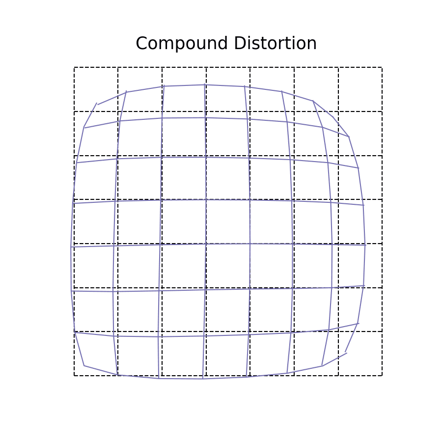
Compound distortions

Typically when we think of distortion, we try to break down the components into their constituent parts to aid our understanding. However, most lens systems in the real world will have what is often referred to as compound distortion. There's no tricks here, it's simply an aggregate effect of all the previous types of distortions in some combination. This kind of distortion is especially prevalent in cameras with compound lenses, or very complicated lens assemblies.

Common Distortion Models

Despite the proliferation and prevalence of cameras and vision-enabled devices over the past century or so, there have been two primary distortion models that have gained widespread adoption to provide correction. We'll go over these, and dive into the math and approach to ground you in these techniques.

Brown-Conrady

Brown-Conrady distortion is probably what most think of as the "standard" radial and tangential distortion model. This model finds its roots in two documents

• Decentering Distortions of Lenses, by Duane C. Brown (link)

• Decentred Lens-Systems, by A. E. Conrady (link)

The documents are quite old and date up to a century ago, but still form the foundation of many of the ideas around characterizing and modeling distortion today!

This model characterizes radial distortion as a series of higher order polynomials:

$$ r = \sqrt{x^2 + y^2} $$

$$ \delta r= k_1 r^3 + k_2 r^5 + k_3 r^7 + ... + k_n r^{n+2} $$

In practice, only the $k_1$ through $k_3$ terms are typically used. For cameras with relatively simple lens assemblies (e.g. only contain one or two lenses in front of the CMOS / CCD sensor), it is often sufficient to just use the $k_1$ and $k_2$ terms.

To relate this back to our image coordinate system (i.e. $x$ and $y$), we usually need to do some basic trigonometry:

$$ \delta x_r = \sin(\psi) \delta r = \frac{x}{r} (k_1r^3 + k_2r^5 + k_3r^7) $$

$$ \delta y_r = \cos(\psi) \delta r = \frac{y}{r} (k_1r^3 + k_2r^5 + k_3r^7) $$

The original documents from Brown and Conrady did not express $\delta r$ in just these terms, and in fact the original documents state everything in terms of "de-centering" distortion broken into radial and tangential components. Symmetric radial distortion as expressed above is a mathematical simplification of the overall power-series describing the radial effects of a lens. The formula we use above is what we call the "Gaussian profile" of Seidel distortion.

Wikipedia has a good summary of the history, but the actual formalization is beyond the scope of what we want to cover here.

Tangential distortion, as characterized by the Brown-Conrady model, is often simplified into the following $x$ and $y$ components. We present these here first as they are probably what most are familiar with:

$$ \delta x_t = p_1(r^2 + 2x^2) + 2p_2xy $$

$$ \delta y_t = p_2(r^2 + 2y^2) + 2p_1xy $$

This actually derives from an even-power series much like the radial distortion is an odd-power series. The full formulation is a solution to the following:

$$ \delta t = P(r) cos(\psi - \psi_0) $$

Where $P(r)$ is our de-centering distortion profile function, $\psi$ is the polar angle of the image plane coordinate, and $\psi_0$ is the angle to the axis of maximum tangential distortion (i.e. zero radial distortion). Expanding this into the general parameter set we use today is quite involved (read the original Brown paper!), however this will typically take the form:

$$ \delta x_t = [p_1(r^2 + 2x^2) + 2p_2xy](1 + p_3r^2 + p_4r^4 + p_5r^6 + ...) $$

$$ \delta y_t = [p_2(r^2 + 2y^2) + 2p_1xy](1 + p_3r^2 + p_4r^4 + p_5r^6 + ...) $$

Because tangential distortion is usually small, we tend to approximate it using only the first two terms. It is rare for de-centering to be so extreme that our tangential distortion requires higher order terms because that would mean that our lens is greatly de-centered relative to our image plane. In most cases, one might ask if their lens should simply be re-attached in a more appropriate manner.

Kannala-Brandt

Almost a century later (2006, from the original Conrady paper in 1919), Juho Kannala and Sami Brandt published their own paper on lens distortions named "A Generic Camera Model and Calibration Method for Conventional, Wide-Angle, and Fish-Eye Lenses". The main contribution of this paper adapts lens distortion modeling to be optimized for wide-angle, ultra wide-angle, and fish-eye lenses. Brown and Conrady's modeling was largely founded on the physics of Seidel aberrations, which were first formulated around 1867 for standard lens physics of the time, which did not include ultra wide and fish-eye lenses.

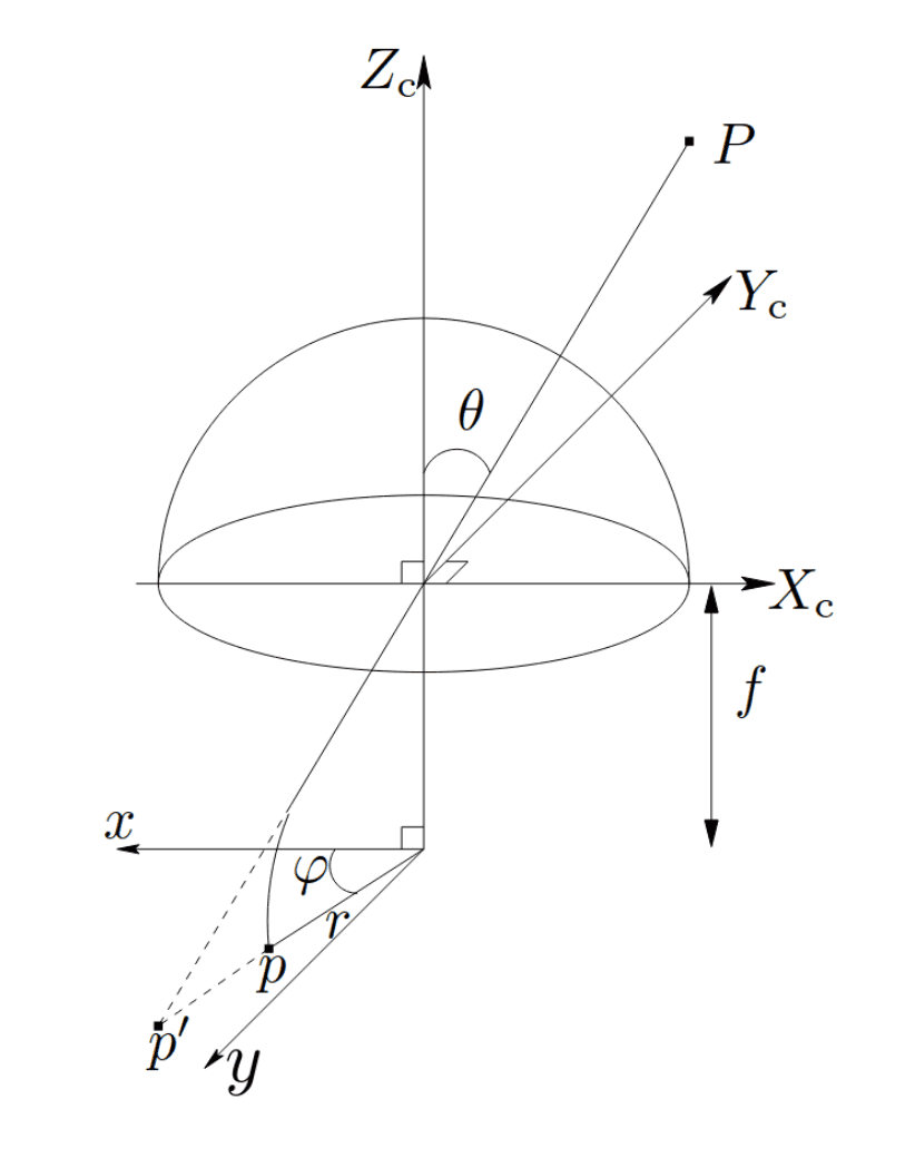
The primary difference that most folks will notice using this model lies in symmetric radial distortion. Rather than characterizing radial distortion in terms of how far a point is from the image center (the radius), Kannala-Brandt characterizes distortion as a function of the incidence angle of the light passing through the lens. This is done because the distortion function is smoother when parameterized with respect to this angle ($\theta$), which makes it easier to model as a power-series:

$$ \theta = \arctan(\frac{r}{f}) $$

$$ \delta r = k_1\theta + k_2\theta^3 + k_3\theta^5 + k_4\theta^7 + ... + k_n\theta^{n+1} $$

Above, we've shown the formula for $\theta$ when using perspective projection, but the main advantage of the Kannala-Brandt model is that it can support different kinds of projection by swapping our formula for $\theta$, which is what makes the distortion function smoother for wide-angle lenses. See the following figure, shared here from the original paper, for a better geometric description of $\theta$:

Kannala-Brandt also aims to characterize other radial (such as asymmetric) and tangential distortions. This is done with the following additional parameter sets:

$$ \delta r_{other} = (l_1\theta + l_2\theta^3 + l_3\theta^5) (i_1 \cos(\psi) + i_2 \sin(\psi) + i_3 \cos(2\psi) + i_4 \sin(2\psi) + ...) $$

$$ \delta t = (m_1\theta + m_2 \theta^3 + m_3 \theta^5)(j_1\cos(\psi) + j_2\sin(\psi) + j_3 \cos(2\psi) + j_4 \sin(2\psi) + ...) $$

Overall, this results in a 23 parameter model! This is admittedly overkill, and the original paper claims as much. These models, unlike the symmetric radial distortion, are an empirical model derived by fitting an N-term Fourier series to the data being calibrated. This is one way of characterizing it, but over-parameterizing our final model can lead to poor repeatability of our final estimated parameters. In practice, most systems will characterize Kannala-Brandt distortions purely in terms of the symmetric radial distortion, as that distortion is significantly larger in magnitude and will be the leading kind of distortion in wider-angle lenses.

Overall, Kannala-Brandt has been chosen in many applications for how well it performs on wide-angle lens types. It is one of the first distortion models to successfully displace the Brown-Conrady model after decades.

All Together Now

Fitting in with our previous camera model, we can formulate this in terms of the collinearity relationship (assuming Brown-Conrady distortions):

$$ \begin{bmatrix} x_i \\ y_i \end{bmatrix} = \begin{bmatrix} f \cdot X_t / Z_t \\ f \cdot Y_t / Z_t \end{bmatrix} + \begin{bmatrix} a_1 x_i \\ 0 \end{bmatrix} + \begin{bmatrix} x_i (k_1 r^2 + k_2r^4+k_3r^6) \\ y_i(k_1r^2 + k_2r^4 + k_3r^6) \end{bmatrix} + \begin{bmatrix} p_1(r^2 + 2x_i^2) + 2 p_2 x_i y_i \\ p_2(r^2 + 2y_i^2) + 2 p_1 x_i y_i \end{bmatrix} $$

or, with Kannala Brandt distortions:

$$ \begin{bmatrix} x_i \\ y_i \end{bmatrix} = \begin{bmatrix} f \cdot X_t / Z_t \\ f \cdot Y_t / Z_t \end{bmatrix} + \begin{bmatrix} a_1 x_i \\ 0 \end{bmatrix} + \begin{bmatrix} \frac{x_i}{r} (k_1 \theta + k_2\theta^3+k_3\theta^5 + k_4\theta^7) \\ \frac{y_i}{r} (k_1 \theta + k_2\theta^3+k_3\theta^5 + k_4\theta^7) \end{bmatrix} $$

Gaussian vs. Balanced Profiles

An astute reader of this article might be thinking right now: "Hey, <library-that-I-use> doesn't use these exact models! That math seems off!" You would mostly be correct there: this math is a bit different from how many popular libraries will model distortion (e.g. OpenCV). Using Brown-Conrady as an example, you might see symmetric radial distortion formulated as so:

$$ \delta r = r + k_1 r^3 + k_2 r^5 + k_3 r^7 $$

or for Kannala-Brandt:

$$ \theta = \arctan(r) $$

$$ \delta r = \theta + k_1 \theta^3 + k_2\theta^5 + k_3\theta^7 + k_4\theta^9 $$

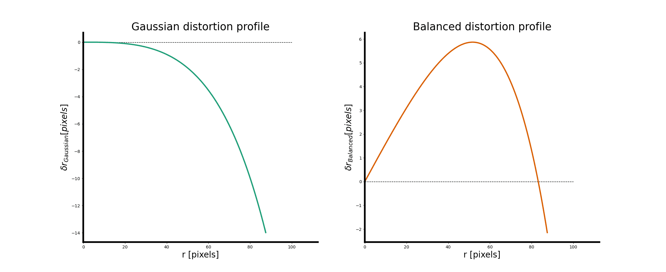
This probably seems quite confusing, because all these formulae are a bit different from the papers presented in this article. Up until now, we have been presenting distortions using what is referred to in photogrammetry as the Gaussian Distortion Profile. Now, the distortions have been re-characterized using what is referred to in photogrammetry as the Balanced Distortion Profile.

See this example comparing two equivalent distortion models. The left describes the Gaussian distortion profile, whereas the right hand side describes a Balanced distortion profile. The distortions are effectively the same, but the model is transformed in the balanced profile scenario; the balanced profile allows us to limit the maximum distortion of the final distortion profile while still correcting for the same effects.

How does one go from one representation to the other? For Brown-Conrady, this is done by scaling the distortion profile by a linear correction:

$$ \delta r_{Balanced} = k_0' r + k_1' r^3 + k_2 'r^5 + k_3'r^7 $$

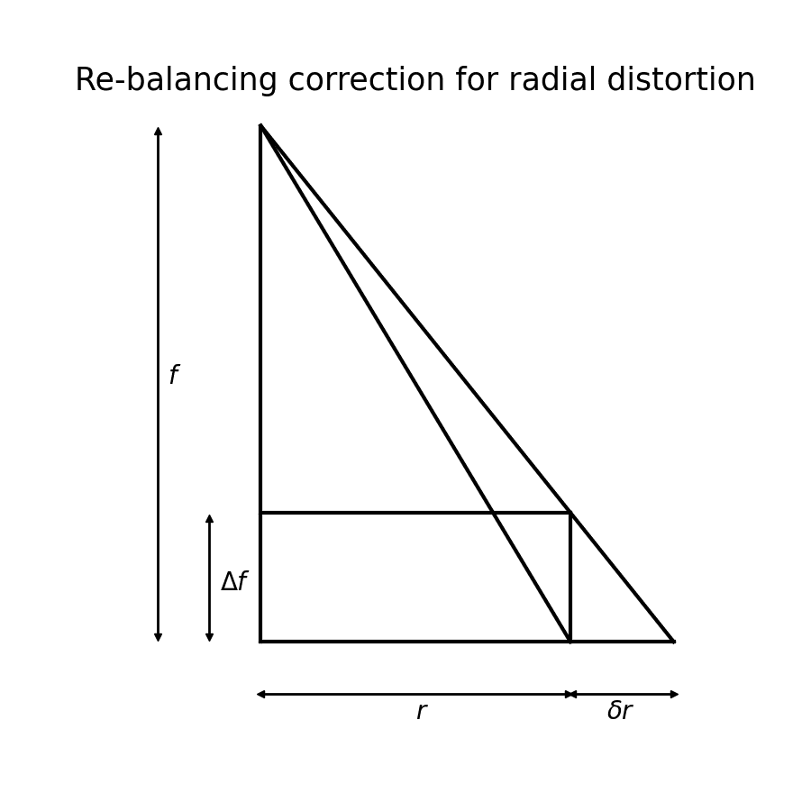
$$ \delta r_{Balanced} = \frac{\Delta f}{f} r + \left(1 + \frac{\Delta f}{f} \right) (k_1r^3 + k_2r^5 + k_3r^7) $$

Note that this linear relationship is derived by similar triangles for Brown-Conrady distortions by the relationships shown in the following figure. Here, we have a set of similar triangles representing the linear correction done to re-balance the Gaussian distortion profile. Re-balancing is used to set the distortion to zero at some radius, or to reconfigure the distortion profile to characterize itself for a virtual focal length.

Historically, the balanced profile was used because distortion was measured manually through the use of mechanical stereoplotters. These stereoplotters had a maximum range in which they could move mechanically, so limiting the maximum value of distortion made practical sense.

Nowadays, with the abundance of computing resources, it is atypical to use mechanical stereoplotters in favor of making digital measurements on digital imagery. There doesn't seem to be a paper trail for why this decision was made, so it could just be a historical artifact. However, doing the re-balancing has some advantages:

1. By parameterizing the model with $\frac{\Delta f}{f} = 1$, as OpenCV does, it makes the math and partial derivatives for self-calibration somewhat easier to implement. This is especially true when using the Kannala-Brandt model, since doing this removes the focal length term from $\theta = \arctan(r),$ which means that there is one less partial derivative to compute.

2. If you keep your entire self-calibration pipeline in units of "pixels" as opposed to metric units like millimeters or micrometers, then the Gaussian profile will produce values for $k_1, k_2, k_3$ that are relatively small. On systems that do not have full IEEE-754 floats (specifically, systems that use 16-bit floats or do not support 64-bit floats at all), this could lead to a loss in precision. Some CPU architectures today do lack full IEEE-754 support (armel, I'm looking at you), so the re-balancing could have been a consideration for retaining machine precision without adding any specialized code. There is no difference in the final geometric precision or accuracy of the self-calibration process as a result of the re-balancing, as it is just a different model.

3. All of the above math is derived from basic lens geometry, and presents a problem if one has to choose a focal length $f$ between $f_x$ and $f_y$! So if you're already using $f_x$ and $f_y$, removing all focal length terms from e.g. Kannala-Brandt distortions may appear to save you from having to make poor approximations of the quantities involved.

Despite these reasons, there is also one very important disadvantage. Notably: the balanced profile with Brown-Conrady distortions introduces a factor of $( 1 + \frac{\Delta f}{f})$ into the determination of $k_1$ through $k_3$. This may not seem like much, but it means that we are introducing a correlation in the determination of these parameters with our focal length. If one chooses a model where $f_x$ and $f_y$ are used, then the choice in parameterization will make the entire calibration unstable, as small errors in the determination of any of these parameters will bleed into every other parameter. This is one kind of projective compensation, and is another reason for why our last article on the subject suggested not to use this parameterization.

It might also seem that with the Kannala-Brandt distortion model, we simplify the math by cancelling out $f$ from our determination of $\theta$. This is true, and it will make the math easier, and remove a focal length term from our determination of the Kannala-Brandt parameters. However, if one chooses a different distortion projection, e.g. orthographic for a fish-eye lens:

$$ \theta_{Gaussian} = \arcsin \left(\frac{r}{f} \right) $$

$$ \theta_{Balanced} = \arcsin(r) $$

Then one will quickly notice that the limit of $\theta_{Balanced}$ is not well defined as $r \rightarrow \infty$, and gives us a value of $(-i)\infty$. As we've tried to separate our focal length from our parameters, we've ended up wading into the territory of complex numbers! Since our max radius and focal length are often proportional, $\theta_{Gaussian}$ does not suffer from the same breakdown in values at the extremes.

It may seem like Kannala-Brandt is a poor choice of model as a result of this. For lenses with a standard field-of-view, the Brown-Conrady model with the Gaussian profile does a better job of determining the distortion without introducing data correlations between the focal length and distortion parameters.

However, the Brown-Conrady model does not accommodate distortions from wide-field-of-view lenses very well, such as when using e.g. fisheye lenses. This is because they were formulated on the basis of Seidel distortions, which do not operate the same way as the field-of-view increases past 90°.

The Kannala-Brandt model, while introducing some correlation between our determination of $f$ and our distortion coefficients $k_1$ through $k_4$, does a better job of mapping distortion with stereographic, orthographic, equidistance, and equisolid projections. As with anything in engineering there are trade-offs, and despite the extra correlations, the Kannala-Brandt model will still often provide better geometric precision of the determined parameters compared to the Brown-Conrady model in many of these scenarios.

As can be seen, chasing simplicity in the mathematical representations is one way in which our choice of model can result in unstable calibrations, or nonsensical math. Given that we want to provide the most stable and precise calibrations possible, we lean towards favoring the Gaussian profile models where possible. It does mean some extra work to make sure the math is correct, but also means that by getting this right once, we can provide the most stable and precise calibrations ever after.

The Bottom Line

We've explored camera distortions, some common models for camera distortions, and explored the ways in which these models have evolved and been implemented over the past century. The physics of optics has a rich history, and there's a lot of complexity to consider when picking a model.

Modeling distortion is one important component of the calibration process. By picking a good model, we can reduce projective compensations between our focal length $f$ and our distortion parameters, which leads to numerical stability in our calibration parameters.