Camera Modeling, Part 1: Focal Length & Collinearity
We explore one of the fundamental aspects of the calibration problem: choosing a model.
Jeremy Steward
Staff Perception Engineer
Jun 10, 2021

Explore our entire Camera Modeling Series:
Part I: Focal Length And Collinearity
Part 2: Introducing Lens Distortion
Part 3: Exploring Distortion and Distortion Models
Part 4: Pinhole Obsession
Part 5: The Deceptively Asymmetric Unit Sphere
If you’d like to be notified of when that next post drops, just follow us on LinkedIn or subscribe to our newsletter.
—
Camera calibration is a deep topic that can be pretty hard to get into. While the geometry of how a single camera system works and the physics describing lens behavior is well-known, camera calibration continues to be mystifying to many engineers in the field.
To the credit of these many engineers, this is largely due to a wide breadth of jargon, vocabulary, and notation that varies across a bunch of different fields. Computer vision seems as if it is a distinct field unto itself, but in reality it was borne from the coalescence of computer science, photogrammetry, physics, and artificial intelligence. As a result of this, the language we use has been adopted from several different disciplines and there's often a lot of cross-talk.
Today, we want to explore one of the fundamental aspects of the calibration problem: choosing a model. More specifically, we're going to take a look at how we model cameras mathematically, and in particular take a look at existing models in use today and some of the different approaches they take. For this first essay, I want to specifically take a look at modeling the focal length, and why the common practice of modeling \(f_x\) and \(f_y\) is sub-optimal when calibrating cameras.
Background
We've covered camera calibration in the past, as well as 3D coordinate transforms. We'll need a basic understanding of these to define what we call the collinearity function. Beyond the above, having some least-squares or optimization knowledge will be helpful, but not necessary.
Let's first start by demonstrating the geometry of the problem:
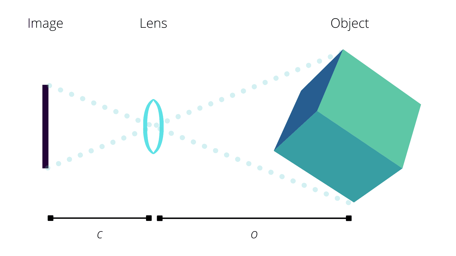
Fig.1: Geometry of how a camera captures an image of an object through a lens following the pinhole projection model.
On the left-hand side we have the image plane. In analogue cameras, this was a strip of photosensitive film stretched across a backplate behind the lens, or a glass plate covered in photosensitive residue. In modern digital cameras, our image "plane" is an array of pixels on a charge-coupled device (CCD).
On the right we have the object we're imaging. The pinhole-projection model of our lens creates two similar triangles in between these. Effectively, for every ray of light that bounces off of the object, there is a straight ray that can be traced back through the lens centre (our pinhole) and directly onto the image plane.
There are two listed distances from the above diagram, namely \(o\) and \(c\):
\(o\) is the distance of our object at the focus point
\(c\) is what we refer to as the principal distance
These distances relate to the lens model that we typically use when doing computer vision or photogrammetry. While the collinearity function that we're going to define is going to be based on a pinhole-projection model, we have to also consider the physics of our lens. Carnegie-Mellon University actually has a really good graphic for demonstrating how and when we can relate our lens geometry to the pinhole-projection model:
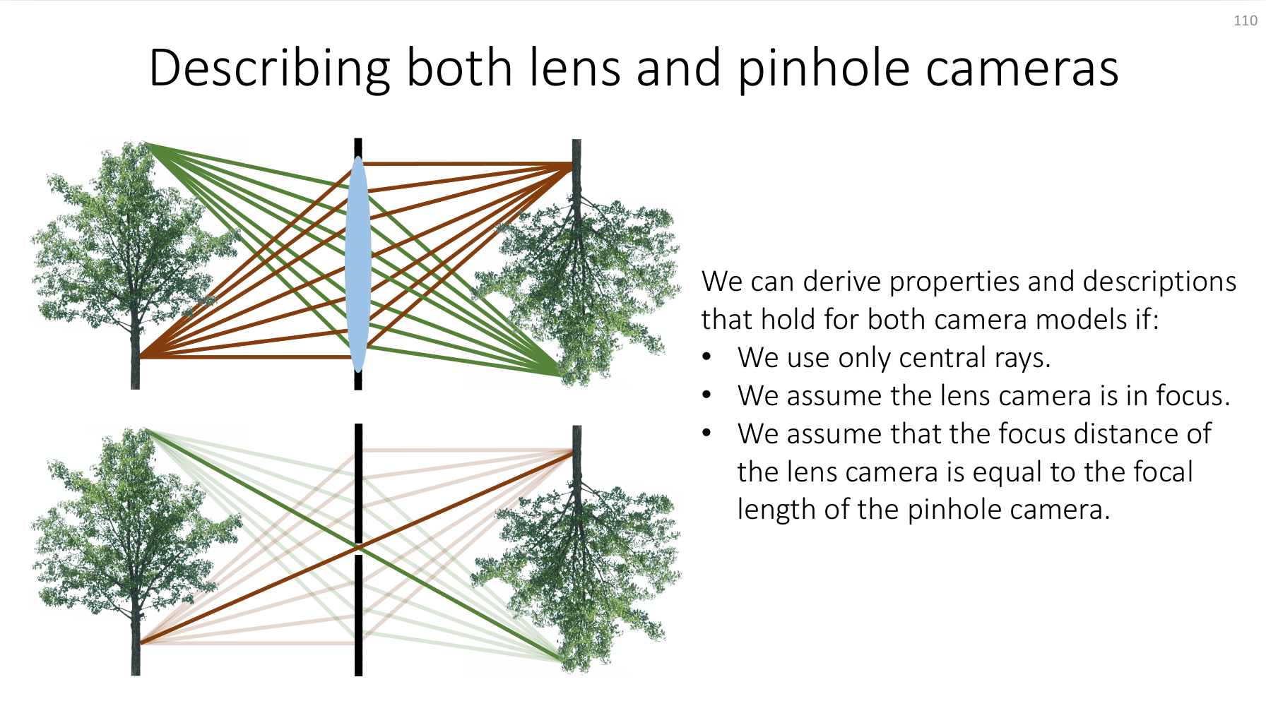
Fig. 2: Slide demonstrating the relationship and assumptions relating the pinhole-projection model to the lens model of our camera. Copyright Ioannis Gkioulekas, CMU, 2020.
Often times there is little distinction made between the principal distance \(c\) and the focal length \(f\) of the camera. This is somewhat of an artifact of the fact that most photogrammetric systems were focused at infinity. If we take the lens equation for a thin convex lens:
$$\frac{1}{f} = \frac{1}{o} + \frac{1}{c}$$
We can see how these values are related. As \(o\) approaches infinity, \(\frac{1}{o}\) approaches zero, which makes the focal length and principal distance the same. Note that if we are calibrating / modeling a camera that is not focused at infinity we can still represent our equations with a single focal length, but we need to be careful about collecting measurements from the image, and ensure that we are only collecting measurements that are in focus.
💡 We're going to take some liberties here regarding focal length / principal distance. With the collinearity function we're going to define, we are exclusively measuring principal distance (the distance between the lens and the image plane). Focal length is different from the principal distance, but the ways in which it can deviate from principal distance are separate from the discussion here regarding \(f_x\) and \(f_y\) as model parameters.
Likewise, for the sake of what we're discussing here we're going to assume that there is no distortion (i.e. that the dotted lines in our first figure are perfectly straight). Distortion doesn't change any of the characteristics we're discussing here with respect to our focal length as it is a different modeling problem.
Collinearity Condition
The graphic above demonstrates the primary relationship that is used when understanding the geometry of how images are formed. In effect, we represent the process of taking an image as a projective coordinate transformation between two coordinate systems. If we were to write this out mathematically, then we would write it as we would any 3D coordinate transformation:
$$\begin{bmatrix} x_i \\ y_i \\ f \end{bmatrix} = \Gamma_{o}^{i} \begin{bmatrix} X_o \\ Y_o \\ Z_o \end{bmatrix}$$
Where \(o\) as a sub/superscript denotes the object space coordinate frame, and \(i\) as a sub/superscript denotes the image plane. In essence, \(\Gamma_{o}^{i}\) is a function that moves a point in object space (the 3D world) to image space (the 2D plane of our image). Note that \(f\) in the above equation is constant for all points, because all points lie in the same image plane.
For the sake of simplicity, let's assume for this modeling exercise that \(\Gamma_o^i\) is known and constant. This lets us substitute the right-hand side of the equation with:
$$\begin{bmatrix} X_t \\ Y_t \\ Z_t \end{bmatrix} = \Gamma_o^i \begin{bmatrix} X_o \\ Y_o \\ Z_o \end{bmatrix}$$
Where subscript \(t\) denotes the transformed point. We can re-order these equations to directly solve for our image coordinates:
$$\begin{bmatrix} x_i / f \\ y_i / f \\ 1 \end{bmatrix} = \begin{bmatrix} X_t / Z_t \\ Y_t / Z_t \\ 1 \end{bmatrix}$$
$$\begin{bmatrix} x_i \\ y_i \end{bmatrix} = \begin{bmatrix} f \cdot X_t / Z_t \\ f \cdot Y_t / Z_t \end{bmatrix}$$
Remember, this is just a standard projective transformation. The focal length \(f\) has to be the same for every point, because every point lies within our ideal plane. The question remains: how do we get \(f_x\) and \(f_y\) as they are traditionally modeled? Well, let's try identifying what these were proposed to fix, and evaluate how that affects our final model.
Arguments of Scale
The focal length \(f\) helps define a measure of scale between our object-space coordinates and our image-space coordinates. In other words, it is transforming our real coordinates in object space (\(X_t\), \(Y_t\), \(Z_t\)) into pixel coordinates in image space (\(x_i\), \(y_i\)) through scaling. How we define our focal length has to be based in something, so let us look at some arguments for how to model it.
Argument of Geometry
From our pinhole projection model, we are projecting light rays from the centre of the lens (our principal point) to the image plane. From a physical or geometric perspective, can we justify both \(f_x\) and \(f_y\)?
The answer is NO, we cannot. The orthonormal distance of the principal point to the image plane is always the same. We know this because for any point \(q\) not contained within some plane \(B\), there can only ever be one vector (line) \(v\) that is orthogonal to \(B\) and intersects \(q\).
From that perspective, there is no geometric basis for having two focal lengths, because our projective scale is proportional to the distance between the image plane and principal point. There is no way that we can have two different scales! Therefore, two focal lengths doesn't make any sense.
💡 Here, I am avoiding the extensive proof for why there exists a unique solution for \(v\) intersecting \(B\) where \(v \perp B\) and \(\forall q \in B : v \not= q\).
If you're really interested, I suggest Linear and Geometric Algebra by Alan Macdonald, it does contain such a proof in its exercises. If you're interested in how point to plane distance is calculated, see this excellent tutorial.
Argument of History
Okay, so perhaps geometrically this lens model is wrong. However, we don't live in a perfect world and our ideal physics equations don't always model everything. Are \(f_x\) and \(f_y\) useful for some other historical reason? Why did computer vision adopt this model in the first place? Well, the prevailing mythos is that it has to do with those darn rectangular pixels! See this StackOverflow post that tries to justify it. This preconception has done considerable damage by perpetuating this model. Rather than place blame though, lets try to understand where this misconception comes from. Consider an array of pixels:

Fig. 3: Two possible arrays of pixels. On the left, we have an ideal pixel grid, where the pixel pitch in x and y is the same (i.e. we have a square pixel). On the right, we have a pixel grid where we do not have equal pitch in x and y (i.e. we have rectangular pixels).
The reason that \(f_x\) and \(f_y\) are used is to try and compensate for the effect of rectangular pixels, as seen in the above figure. From our previous equations, we might model this as two different scales for our pixel sizes in the image plane:
$$\begin{bmatrix} x_i \cdot \rho_x \\ y_i \cdot \rho_y \end{bmatrix} = \begin{bmatrix} f \cdot X_t / Z_t \\ f \cdot Y_t / Z_t \end{bmatrix}$$
Where \(\rho_x\) is the pixel pitch (scale) of pixels in the \(x\)-direction, and \(\rho_y\) is the pixel pitch (scale) of pixels in the \(y\)-direction. Eventually we want to move these to the other side as we did before, which gives us:
$$\begin{bmatrix} x_i \\ y_i \end{bmatrix} = \begin{bmatrix} \frac{f}{\rho_x} \cdot X_t / Z_t \\ \frac{f}{\rho_y} \cdot Y_t / Z_t \end{bmatrix}$$
If we then define:
$$f_x = f / \rho_x$$
$$f_y = f / \rho_y$$
Then we have the standard computer vision model of the collinearity equation. From the perspective of what's going one with this example, it isn't completely wild to bundle these together. Any least-squares optimization process would struggle to estimate the focal length and pixel pitch as separate quantities for each dimension. From that perspective, it seems practical to bundle these effects together into \(f_x\) and \(f_y\) terms. However, now we've tried to conflate our model between something that does exist (different pixel sizes) with something that does not exist (separate distances from the image plane in the \(x\)- and \(y\)-directions).
But this assumes that pitch is applied as a simple multiplicative factor in this way. Modeling it this way does not typically bode well for the adjustment. The immediate question is then: is there a better way to model this? Can we keep the geometric model and still account for this difference? The answer, unsurprisingly, is yes. However, to get there we first have to talk a bit more about this scale difference and how we might model it directly in the image plane.
Differences in Pixel Pitch
Whenever adding a new term to our model, that term must describe an effect that is observable (compared to the precision of our measurements in practice). It doesn't make sense to add a term if it doesn't have an observable effect, as doing so would be a form of over-fitting. This is a waste of time, sure, but it also risks introducing new errors into our system, which is not ideal.
So the first questions we have to ask when thinking about pixel pitch is: how big is the effect, and how well will we able to observe it?
This effect appears as if there is a scale difference in \(x\) and \(y\). This could be caused by one of a few factors:
Measured physical differences due to rectangular pixels.
Differences between the clock frequencies of the analogue CCD / CMOS clock and sampling frequency of the Digital-Analog Converter (DAC) in the frame grabber of the camera hardware.
The calibration data set has or had an insufficient range of \(Z_o\) values in the set of object-space points. Put more directly, this is a lack of depth-of-field in our object points. Often this occurs when all your calibration targets are within a single plane (such as when you use just a checkerboard, and all your points are in a single plane).
Measured Physical Differences
We've already discussed what physical differences in the pixel size looks like (i.e. rectangular pixels). In general, this is fairly rare. Not because rectangular pixels don't exist, but because measuring each pixel is fairly difficult: pixels are really small. For some cameras, this isn't as difficult; many time-of-flight cameras, for example, can have pixels with a pitch of approximately 40μm (a relatively large size). But for many standard digital cameras, pixel sizes range from 3μm - 7μm.
If we're trying to estimate differences between the pitch in \(x\) and \(y\), how large do they have to be before we notice them? If the difference was approximately 10% of a pixel, then for a 3μm pixel we'd need to be able to observe changes in the image plane of approximately 0.3μm. This is minuscule. The difference in pixel size would have to be much larger in order for us to actually observe such a difference.
Clock-frequency Differences
Scale differences can also "appear" out of our data due to frequency differences between the frequency of the CCD pixel clock and the sampling frequency of the DAC in the frame grabber of the digital camera. For a single row of pixels, this frequency difference would look similar to:

Fig. 4: Example of a signal being read out along a line of pixels. Each vertical colored line is a pixel. In the top version, the CCD pixel clock is what determines the frequency of readout. In the bottom, the DAC sampling frequency is used, which produces a perceived difference in the final pixel pitch.
The purple lines are the true locations in the signal that we should be sampling, but the orange lines are where we actually sample. We can see that the sampled pixels (in orange) have a different pitch. The columns (not shown here) are sampled evenly at the original pixel pitch, but the rows were sampled incorrectly at the scaled pixel pitch. As a result, we would observe two different scales in the \(x\) and \(y\) directions.
This effect can be overcome today with pixel-synchronous frame grabbing (e.g. in a global shutter synchronous camera) or on board digital-analog conversion. However, this mechanic isn't in every camera, especially when it comes to cheap off-the-shelf cameras.
💡 It may also exist due to the CCD array configuration in hardware, if pixels have different spacing in \(x\) and \(y\), but that again goes back to the first point where we have to be able to measure these physical differences somehow. Nonetheless, the effect is the same on the end result (our pixel measurements).
The above "array configuration" problem is common when for example we "interpolate" our pixel data from a Bayer pattern of multiple pixels. This makes the spacing uneven as we often have more of one color pixel (green) than we do of other kinds of pixels (red, blue). See our guest post on OpenCV's blog for more info.
Insufficient Depth-of-Field
Even if we assume that our hardware was perfect and ideal, and that our pixels were perfectly square, we might still observe some scale difference in \(x\) and \(y\). This could be because our calibration data set comprises only points in a single plane, and we lack any depth-of-field within the transformation.
Unfortunately, this ends up appearing as a type of projective compensation as a result of the first derivative of our ideal model. Projective compensation can occur when two parameters (e.g. in a calibration) influence each other's values because they cannot be estimated independently.
This is the point where we would be going off into the weeds of limits and derivatives, so we will leave the explanation at that for now. The important consideration is that even in an ideal world, we might still actually observe this effect, and so we should model it!
Scale and Shear in Film
So we've now ascertained that modeling these scale differences as a factor of \(f_x\) and \(f_y\) doesn't make sense geometrically. However, that doesn't mean that we aren't going to see this in practice, even if our camera is close to perfect. So how are we to model this scale effect? Fortunately, the past has an answer! Scale (and shear) effects were very common back when cameras used to be analogue and based on physical film.
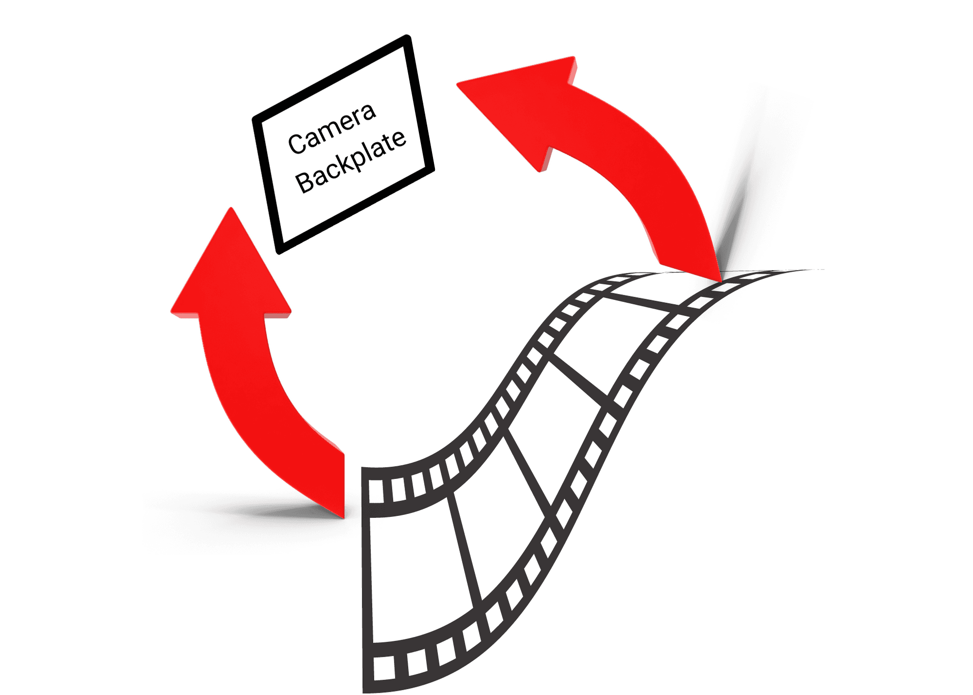
Fig. 5: Example of how film is stretched across a backplate in a traditional analogue camera.
Consider the above scenario where we are stretching a film of some material across a backplate in the camera. Tension across the film being stretched over the backplate was in the \(x\) direction, but not the \(y\) direction. This difference in tension could cause a scale difference in the final developed image, as that tension is not present when the film is developed.
Back then, shear effects were also modeled in addition to scale. This effectively meant that the tension along one diagonal of the image was not equal to the tension along the other diagonal. This would result in a warping or shear effect in the final image plane. Nowadays, this would mean that our pixels are not a rectangle or a square, but rather some rhombus. This isn't particularly realistic for modern digital cameras, so we ignore it here.
In any case, we end up with the following additional parameter to account for scale differences.
$$\begin{bmatrix} x_i - a_1x_i \\ y_i \end{bmatrix} = \begin{bmatrix} f \cdot X_t / Z_t \\ f \cdot Y_t / Z_t \end{bmatrix}$$
Where \(a_1\) is a multiplicative factor applied to the \(x\) coordinate. This model has a foundation in the literature dating back decades (see equation 9, however there it is referred to as \(b_1\) instead of \(a_1\)).
Is There A Difference Between These Two Models?
Mathematically, yes! This different model has a couple things going for it:
We maintain the original projective geometry of the collinearity function.
We model scale differences in \(x\) and \(y\) in the image plane directly.
Our calibration process has better observability between \(f\) and \(a_1\) because we aren't conflating different error terms together and are instead modeling them independently based off a physical model of how our system behaves.
That last point is the most important. Remember the original systems of equations we ended up with:
$$\frac{x_i}{f} = \frac{X_t}{Z_t}$$
$$\frac{y_i}{f} = \frac{Y_t}{Z_t}$$
From this, we bundled together the pixel pitch as if that was the only effect. This was possible because when optimizing, it's not possible to observe differences between two multiplicative factors, e.g.:
$$w = r\cdot s\cdot v$$
If we know \(v\) and \(w\) as say, 2 and 8 respectively, there's no way for us to cleanly estimate \(r\) and \(s\) as separate quantities. Pairs of numbers that would make that equality true could be 2 and 2, or 4 and 1, or any other multitude of factors. In the same way, if we try to reconstruct our original definitions for \(f_x\) and \(f_y\), we would get:
$$x_i - a_1x_i = f(X_t / Z_t)$$
$$x_i (1 - a_1) = f(X_t/Z_t)$$
$$f_x = f /(1 - a_1)$$
and similarly for \(y\), where we would get:
$$f_y = f /(1 - 0)$$
However, remember that this only works if scale differences are the only error factor in our image plane. This is not often the case. If we have additional errors \(\epsilon_x\) and \(\epsilon_y\) in our system, then instead we would get:
$$f_x = f / (1 + a_1 + \frac{\epsilon_x}{x_i})$$
$$f_y = f / (1 + \frac{\epsilon_y}{y_i})$$
Rather than modeling our calibration around the physical reality of our camera systems, this bundles all of our errors into our focal length terms. This leads to an instability in our solution for \(f_x\) and \(f_y\) when we perform a camera calibration, as we end up correlating scene or image-specific errors of the data we collected (that contain \(1/x_i\) or \(1/y_i\)) into our solution for the focal length. If we don't use \(f_x\) and \(f_y\) , and \(\epsilon_x\) and \(\epsilon_y\) are uncorrelated (i.e. independent variables) then we can easily observe \(f\) independently. In doing so, we have a stronger solution for our focal length that will generalize beyond just the data set that was used in the calibration to estimate it.
Now obviously, you would say, we want to model \(\epsilon_x\) and \(\epsilon_y\), so that these are calibrated for in our adjustment. Modeling our system to match the physical reality of our camera geometry in a precise way is one key to removing projective compensation between our parameters and to estimate all of our model parameters independently. By doing so, we avoid solving for "unstable" values of \(f_x\) and \(f_y\), and instead have a model that generalizes beyond the data we used to estimate it.
At the end of the day, it is easier to get a precise estimate of:
$$\begin{bmatrix} x_i \\ y_i \end{bmatrix} = \begin{bmatrix} f \cdot X_t / Z_t \\ f \cdot Y_t / Z_t \end{bmatrix} + \begin{bmatrix} a_1 x_i \\ 0 \end{bmatrix} $$
as a model, over:
$$\begin{bmatrix} x_i \\ y_i \end{bmatrix} = \begin{bmatrix} f_x \cdot X_t / Z_t \\ f_y \cdot Y_t / Z_t \end{bmatrix}$$
Conclusion
Hopefully we've demonstrated why the classical use of \(f_x\) and \(f_y\) in most calibration pipelines is the wrong model to pick. There's always different abstractions for representing data, but using a single focal length term better matches the geometry of our problem, and doesn't conflate errors in the image plane (scale differences in \(x\) and \(y\) directions of that plane) with parameters that describe geometry outside that image plane (the focal distance). Most importantly, a single focal length avoids projective compensation between the solution of that focal length and measurement errors in our calibration data set.
Modeling sensors is a difficult endeavour, but a necessary step for any perception system. Part of what that means is thinking extremely deeply about how to model our systems, and how to do so in the way that best generalizes across every scene, environment, and application. To do that, though, you'll need rock-solid calibration.
Lucky for you, you have MetrICal, Tangram Vision's premier multi-modal calibration suite for cameras, IMUs, LiDAR, radar, and chassis registration. MetriCal does everything here for you, and a whole lot more, making calibration a breeze. Download MetriCal today and get calibrating!
—
Edits:
June 2, 2025: Removed reference to the Tangram Vision SDK. Added link to MetriCal Installation page.


