Calibration From Scratch Using Rust: Part 3 of 3

In Part I and Part II of our series, we covered the theory, principles, mathematics, and some of the code required to create your own camera calibration module. If you have not yet read Part I and II, we strongly recommend doing so to ground yourself in these elements before exploring Part III, where we apply this to creating a model.

Because the Tangram Vision SDK is written in Rust (with wrappers for C and ROS, of course), we'll demonstrate how to create a calibration module in Rust. We’ll be using the NAlgebra linear algebra crate and the argmin optimization crate. You can follow along here, or with the full codebase at the Tangram Visions Blog repository. Let's get started.

Putting it Together in Rust

Generating Data

In this tutorial we aren’t going to work with real images, but rather synthetically generate a few sets of image points using ground truth transforms and camera parameters.

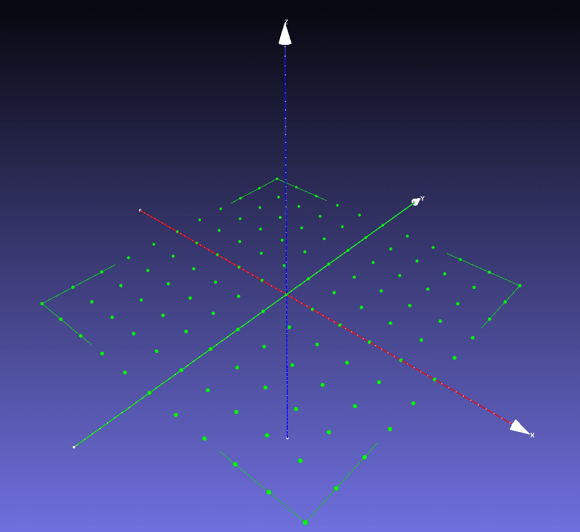
To start we’ll generate some model points. The planar target lies in the XY plane. It will be a meter on each edge.

```rust

let mut source_pts: Vec<na::Point3<f64>> = Vec::new();
for i in -5..6 {
   for j in -5..6 {
       source_pts.push(na::Point3::<f64>::new(i as f64 * 0.1, j as f64 * 0.1, 0.0));
   }
}

```

Then we’ll generate a few arbitrary camera-from-model transforms and some camera parameters.

```rust

let camera_model = na::Vector4::<f64>::new(540.0, 540.0, 320.0, 240.0); // fx, fy, cx, cy
let transforms = vec![
   na::Isometry3::<f64>::new(
       na::Vector3::<f64>::new(-0.1, 0.1, 2.0),//translation
       na::Vector3::<f64>::new(-0.2, 0.2, 0.2),//rotation
   ),
   na::Isometry3::<f64>::new(
       na::Vector3::<f64>::new(-0.1, -0.1, 2.0),
       na::Vector3::<f64>::new(0.2, -0.2, 0.2),
   ),
   na::Isometry3::<f64>::new(
       na::Vector3::<f64>::new(0.1, 0.1, 2.0),
       na::Vector3::<f64>::new(-0.2, -0.2, -0.2),
   ),
];

```

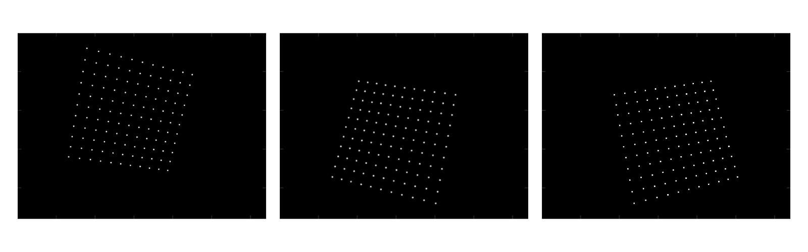
Finally we’ll generate the imaged points by applying the image formation model.

```rust

let transformed_pts = transforms
   .iter()
   .map(|t| source_pts.iter().map(|p| t * p).collect::<Vec<_>>())
   .collect::<Vec<_>>();

let imaged_pts = transformed_pts
   .iter()
   .map(|t_list| {
       t_list
           .iter()
           .map(|t| project(&camera_model, t))
           .collect::<Vec<na::Point2<f64>>>()
   })
   .collect::<Vec<_>>();

```

Building the Optimization Problem

We’re going to use the `argmin` crate to solve the optimization problem. To build your own problem with `argmin`, you make a struct which implements the `ArgminOp` trait. The struct holds the data we're processing. Depending on the optimization algorithm you select, you’ll have to implement some of the trait’s functions. We’re going to use the Gauss-Newton algorithm which requires that we implement `apply()` which calculates the residual vector and `jacobian()` which calculates the Jacobian. The implementations for each are in the previous sections.

```rust

struct Calibration<'a> {
   model_pts: &'a Vec<na::Point3<f64>>,
   image_pts_set: &'a Vec<Vec<na::Point2<f64>>>,
}

```

During the optimization problem, the solver will update the parameters. The parameters are stored in a flat vector and thus it's useful to make a function that converts the parameter vector into easily-used objects for calculating the residual and Jacobian in the next iteration. Here's how we've done it:

```rust

impl<'a> Calibration<'a> {
   /// Decode the camera model and transforms from the flattened parameter vector
   fn decode_params(
&self,
       param: &na::DVector<f64>,
   ) -> (na::Vector4<f64>, Vec<na::Isometry3<f64>>) {
       let camera_model: na::Vector4<f64> = param.fixed_slice::<4, 1>(0, 0).clone_owned();
       let transforms = self
           .image_pts_set
           .iter()
           .enumerate()
           .map(|(i, _)| {
               let lie_alg_transform: na::Vector6<f64> =
                   param.fixed_slice::<6, 1>(4 + 6 * i, 0).clone_owned();
               exp_map(&lie_alg_transform)
           })
           .collect::<Vec<_>>();
       (camera_model, transforms)
   }
}

```

Running the Optimization Problem

Before we run the optimization problem we’ll have to initialize the parameters with some reasonable guesses. In the code block below, you'll see that we input four values for \\(f_x, f_y, c_x,\\) and \\(c_y\\).

```rust

let mut init_param = na::DVector::<f64>::zeros(4 + imaged_pts.len() * 6);

// Arbitrary guess for camera model
init_param[0] = 1000.0; // fx
init_param[1] = 1000.0; // fy
init_param[2] = 500.0; // cx
init_param[3] = 500.0; // cy

// Arbitrary guess for poses (3m in front of the camera with no rotation)
let init_pose = log_map(&na::Isometry3::translation(0.0, 0.0, 3.0));

// Populate poses with guess
init_param
   .fixed_slice_mut::<6, 1>(4, 0)
   .copy_from(&init_pose);
init_param
   .fixed_slice_mut::<6, 1>(4 + 6, 0)
   .copy_from(&init_pose);
init_param
   .fixed_slice_mut::<6, 1>(4 + 6 * 2, 0)
   .copy_from(&init_pose);

```

Next we build the `argmin` "executor" by constructing a solver and passing in the `ArgminOp` struct.

```rust

let cal_cost = Calibration {
   model_pts: &source_pts,
   image_pts_set: &imaged_pts,
};
let solver = argmin::solver::gaussnewton::GaussNewton::new()
   .with_gamma(1e-1)
   .unwrap();
let res = Executor::new(cal_cost, solver, init_param)
   .add_observer(ArgminSlogLogger::term(), ObserverMode::Always)
   .max_iters(2000)
   .run()
   .unwrap();

eprintln!("{}\\n\\n", res);
eprintln!("ground truth intrinsics: {}", camera_model);
eprintln!(
   "optimized intrinsics: {}",
   res.state().best_param.fixed_slice::<4, 1>(0, 0)
);

```

After letting the module run for over 100 iterations, the cost function will be quite small and we can see that we converged to the right answer.

```rust

ground truth intrinsics:
 ┌     ┐
 │ 540 │
 │ 540 │
 │ 320 │
 │ 240 │
 └     ┘

optimized intrinsics:
 ┌                    ┐
 │  539.9999999989419 │
 │    539.99999999895 │
 │ 320.00000000071225 │
 │  240.0000000009506 │
 └                    ┘

```

Concluding Part III

So there you have it - the theory and the execution of a built-from-scratch calibration module for a single sensor. You can revisit Part I and Part II to review what we explored prior to demonstrating execution of the model above.

As we noted at the end of Part II, creating a calibration module for sensors is no trivial task. The simplified module and execution we've described in these two posts provide the building blocks for a single camera approach, without optimizations for calibration time, compute resources, or environmental variability. Adding these factors, and expanding calibration routines to multiple sensors, makes the calibration challenge significantly more difficult to achieve. That's why multi-sensor, multi-modal calibration is a key part of the Tangram Vision SDK. You can request access to the Tangram Vision SDK and test it on up to five device instances at no cost.

‍