Calibration From Scratch Using Rust, Part 2: Zhang's Method
Explore the complex mathematics required for sensor and camera calibration.
Paul Schroeder
Staff Perception Engineer
Jun 1, 2021

Explore our entire Calibration From Scratch Series:
If you’d like to be notified of when that next post drops, just follow us on LinkedIn or subscribe to our newsletter.
—
Zhang's Method
Many camera calibration algorithms available these days are some variant of a method attributed to Zhengyou Zhang (A Flexible New Technique for Camera Calibration by Zhengyou Zhang). If you've calibrated with a checkerboard using OpenCV, this is the algorithm you're using.
Put briefly, Zhang’s method involves using several images of a planar target in various orientations relative to the camera to estimate the camera parameters. The planar target has some sort of automatically-detectable features that provide known data correspondences for the calibration system. These are usually grids of checkerboard squares or small circles. The planar target has known geometry and thus the point features on the target are described in some model or object coordinate system; these are often points on the XY plane, but that’s an arbitrary convention.
Detecting and localizing these features is a topic in itself. We won't be covering it here.
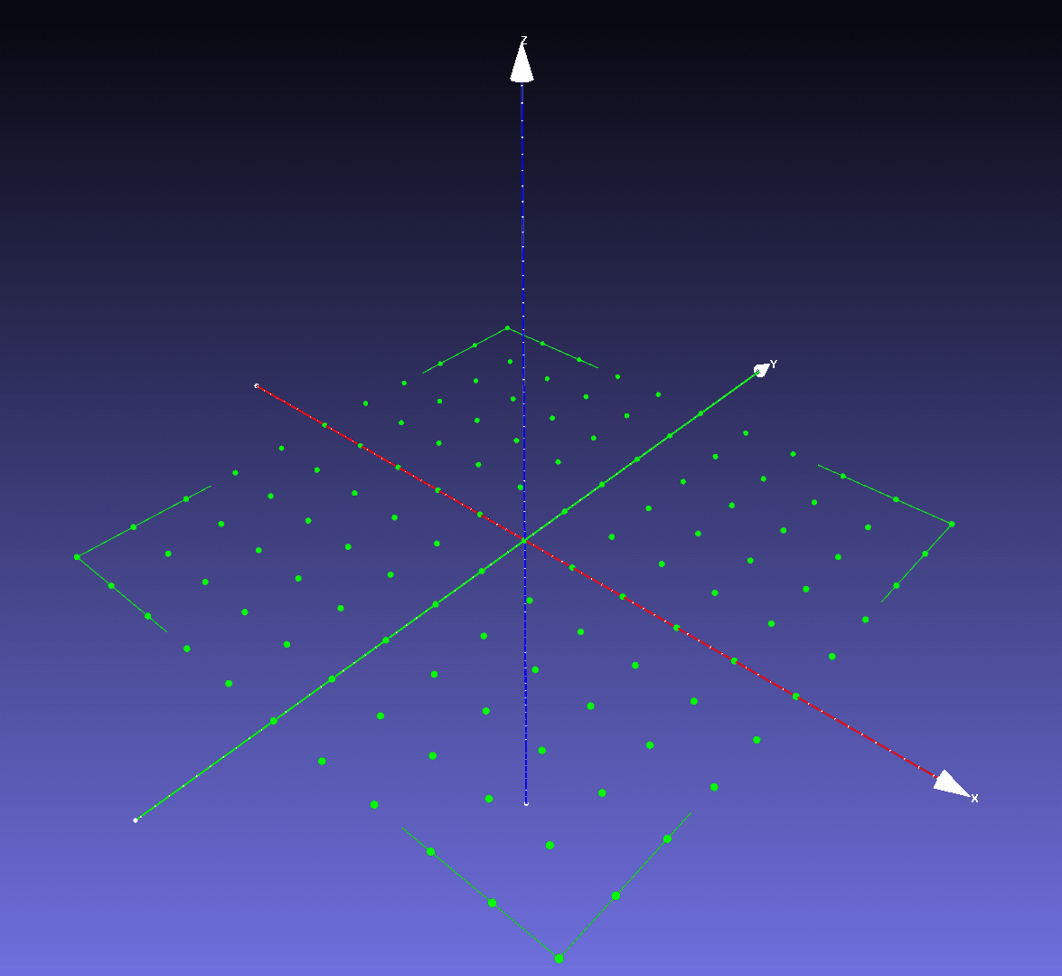
Figure 1: An example planar target with points in a model coordinate system .
From Object to Image Coordinates
Before getting into the algorithm, it’s useful to briefly revisit image formation. Recall that in order to apply a projection model, we need to be in the camera’s coordinate system (i.e. camera at the origin, typically camera looks down the +Z axis etc.). We only know the target’s dimensions in its coordinate system; we don’t know precisely where the target is relative to the camera. Let’s say that the there is a rigid body transform that maps points in the model coordinate system to the camera coordinate system: \(\Gamma_{model}^{camera}\) We can then write out the image formation equation for a given model point:
$$m_i=P(\Gamma_{model}^{camera}\cdot M_i; \{ \theta_k \})$$
Where:
\(m_i\) is the ith imaged model point (a 2-Vector in pixels)
\(m_i=P(\Gamma_{model}^{camera}\cdot M_i; \{\theta_k\})\) is the projection model, with \(k\) parameters \( {\theta_k} \). This will be the pinhole model in further examples.
\(\Gamma_{model}^{camera}\cdot M_i\) is the ith model point transformed into the camera’s coordinate frame.
We don't know this transform and moreover, we need one such transform for each image in the calibration data-set because either the camera or checkerboard or both can and should move between image captures. Thus we'll have to add these transforms to the list of things to estimate.
Cost Function
Ultimately the algorithm boils down to a non-linear least squares error minimization task. The cost function is based around reprojection error which broadly refers to the error between an observation and the result of passing the corresponding model point through the projection model. This is calculated for every combination of model point and image. Assuming we have good data and the model is a good fit for our camera, if we've estimated the parameters and transforms correctly, we should get near-zero error.
$$\{\theta_k\}, \{\Gamma_{model}^{camera_j} \}=\underset{\{\theta_k\}, \{\Gamma_{model}^{camera_j} \}}{\operatorname{argmin}}\sum_{i}^{m}\sum_{j}^{n}\lvert \lvert P(\Gamma_{model}^{camera_j}\cdot M_i; \{\theta_k\})-m_i \rvert \rvert_{2}^{2}$$
Non-Linear Least Squares Minimization
It should be clear from the above cost function that this is a least squares problem. In general, the cost function will also be nonlinear, meaning there won’t be a closed form solution and we’ll have to rely on iterative methods. There’s a great variety of nonlinear least squares solvers out there. Among them are:Gauss-Newton(a good place to start if you want to implement one of these yourself),Levenberg-Marquardt, andPowell’s dog leg method. There are a number of libraries that can implement these algorithms. For any of these algorithms to work you must provide them with (at a minimum) two things: the residual (i.e. the expression inside the \(\lvert\lvert\cdot\rvert\rvert_2^2\) part of the cost function, and theJacobian(matrix of first partial derivatives) of the residual.
Before we get into calculating these quantities, it’s useful to reshape the cost function so that we have one large residual vector. The trick is to see that taking the sum of the norm-squared of many small residual vectors is the same as stacking those vectors into one large vector and taking the norm-squared.
$$\sum_{i}^{m}\sum_{j}^{n}\lvert \lvert r_{ij} \rvert \rvert_{2}^{2}=\lvert \lvert \begin{bmatrix}r_{00} & \dots &r_{0m} & r_{10} & \dots &r_{nm}\end{bmatrix}^T\rvert \rvert_{2}^{2}$$
Calculating the residual is relatively straightforward. You simply apply the projection model and then subtract the observation, stacking the results into one large vector. We'll demonstrate calculating the residual in the code block below:
The Jacobian
The Jacobian is a bit more complicated. In this scenario, we’re interested in the Jacobian of the stacked residual vector with-respect-to the unknown parameters that we’re optimizing. By convention this Jacobian will have the following dimensions: \\(J\in\mathbb{R}^{2NM\times(6M+4)}\\). The number of rows is the dimension of the output of the function which is 2NM because we have NM residuals each of which is 2D (because they’re pixel locations). The number of columns is the number of parameters we're estimating and has two parts. The 4 represents the four camera parameters we’re estimating. This number will change with the camera model. The 6M for M images represents the camera-from-model transforms describing the relative orientation of the camera and planar target in each image. A 3D transformation has six degrees of freedom.
The Jacobian can be thought of as being built up from "residual blocks". A residual block is one residual's contribution to the Jacobian and in this case a residual block is a pair of rows (pair because the residual is 2D). While the camera model is part of every residual block, each residual block only has one relevant transform. This results in the Jacobian having a sparse block structure where, for a given residual block, only a few columns, those relating to the camera parameters and the transform at hand, will be non-zero. For larger calibration problems or least squares problems in general it can be beneficial to leverage the sparse structure to improve performance.
$$J = \begin{bmatrix}-&J_{r_{00_{uv}}}&-\\ -&\vdots&- \\ -&J_{r_{mn_{uv}}}&-\end{bmatrix}=\begin{bmatrix}J_{r_{00_{uv}\theta_k}}&J_{r_{00_{uv}T_0}}& \textbf{0} &\dots& \textbf{0} \\ \vdots \\J_{r_{m0_{uv}\theta_k}}&J_{r_{m0_{uv}T_0}}& \textbf{0} &\dots& \textbf{0} \\J_{r_{01_{uv}\theta_k}}&\textbf{0}&J_{r_{01_{uv}T_1}} &\dots& \textbf{0} \\ \vdots &\vdots&\vdots &\ddots &\vdots \\J_{r_{mn_{uv}{\theta_k}}}&\textbf{0}&\dots & \textbf{0} & J_{r_{mn_{uv}T_n}}\end{bmatrix}$$
\(J_{r_{ij_{uv}}}\in\mathbb{R}^{2\times(6M+4)}\) is a pair of rows corresponding to the ith model point and jth image. It's made up of smaller Jacobians that pertain to the camera parameters or one of the transforms.
\(J_{r_{ij_{uv}\theta_k}}\in\mathbb{R}^{2\times4}\) is the Jacobian of the residual function of the ith model point and jth image with respect to the four camera parameters.
\(J_{r_{ij_{uv}T_j}}\in\mathbb{R}^{2\times6}\) is the Jacobian of the residual function of the ith model point and jth image with respect to the jth transform.
\(\textbf{0}\in\mathbb{R}^{2\times6}\) is the Jacobian of the residual function of the any model point and jth image with respect to the any transform but the jth one. Only one transform appears in the residual equation at a time, so Jacobians for other transforms are always zero.
So now we know the coarse structure, but to fill out this matrix, we’ll need to derive the smaller Jacobians.
Jacobian of the Projection Function
Let’s define the residual function with respect to the parameters:
$$r(\theta_k)\in\mathbb{R}^2=P(\Gamma_{model}^{camera_j}\cdot M_i; \{\theta_k\})-m_i$$
$$\theta_k = [f_x, f_y, c_x, c_y]^T \in \mathbb{R}^4$$
We’re looking for the Jacobian with the partial derivatives with-respect-to the model coefficients. Since there are four inputs and two outputs, we expect a Jacobian \(J_{r\theta}\in\mathbb{R}^{2\times4}\)
$$J_{r\theta}=\begin{bmatrix}\frac{\delta P(X;\theta)}{\delta f_x}&\frac{\delta P(X;\theta)}{\delta f_y}&\frac{\delta P(X;\theta)}{\delta c_x}&\frac{\delta P(X;\theta)}{\delta c_y}\end{bmatrix}=\begin{bmatrix} \frac{x}{z} & 0 &1&0 \\ 0 & \frac{y}{z} & 0 &1 \end{bmatrix}$$
$$\textrm{where } X = \begin{bmatrix}x&y&z\end{bmatrix}^T=\Gamma_{model}^{camera_j}\cdot M_i$$
Jacobian of the Transformations
Because of the complexity of this topic, we're necessarily streamlining a few details for the sake of brevity. There’s a broad topic in computer vision, computer graphics, physics, etc. of how to represent rigid body transforms. Common representations are: 4x3 matrices used with homogeneous points, separate rotation matrix and translation vector pairs, quaternions and translation pairs and Euler angles and translation pairs. Each of these have benefits and drawbacks but most of them are difficult to use in optimization problems. The main reason is that most of the rotation representations have additional constraints. For example, a rotation matrix must be orthogonal and a quaternion must be a unit quaternion. It’s difficult to encode these constraints in the optimization problem without adding a lot of complexity. Without the constraints the optimization is free to change the individual elements of the rotation such that the constraint is no longer maintained. For example, with a rotation matrix representation, you may end up learning more general non-rigid linear transformation that can stretch, skew, scale etc.
For this optimization we’re going to represent the transformations as 6D elements of a “Lie Algebra”. Unlike the other representations, all values of this 6D vector are valid rigid-body transforms. I’m going to defer to other texts to explain this topic, as they can go pretty deep. The texts explain how to convert to (an operation called the “log map”) a “lie algebra” element and convert from (an operation called the “exponetial map”) a “lie algebra”, as well as some Jacobians:
A micro Lie theory for state estimation in robotics by Solà et al
A tutorial on SE(3) transformation parameterizations and on-manifold optimization by Blanco-Claraco
We’ll need the Jacobian with the partial derivatives with-respect-to the six transform parameters. Since there are six inputs and two outputs, we expect a Jacobian \(J_{rT}\in\mathbb{R}^{2\times6}\).
Since we’re observing the effects of the transformation through the projection function we’ll have to employ the Chain rule:
$$J_{r\Gamma}=\frac{\delta r}{\delta \Gamma}=\frac{\delta P(\Gamma\cdot M)}{\delta \Gamma}=\frac{\delta P(X)}{\delta X}\rvert_{X=\Gamma\cdot M}\cdot\frac{\delta \Gamma\cdot M}{\delta \Gamma}$$
So our Jacobian is written as a product of two other Jacobians. The first term is the matrix of partial derivatives of the projection function with-respect-to the point-being-projected (evaluated at the transformed point) \(J_{PX}\in\mathbb{R}^{2\times3}\).
$$J_{PX}=\begin{bmatrix}\frac{\delta P(X)}{\delta x}&\frac{\delta P(X)}{\delta y}&\frac{\delta P(X)}{\delta z}\end{bmatrix}=\begin{bmatrix} \frac{f_x}{z} & 0 &-\frac{f_x x}{z^2} \\ 0&\frac{f_y}{z} &-\frac{f_y y}{z^2} \end{bmatrix}$$
$$\textrm{where } X = \begin{bmatrix}x&y&z\end{bmatrix}^T=\Gamma_{model}^{camera_j}\cdot M_i$$
The second term is the matrix of partial derivatives of a point being transformed with-respect-to the transform: \(J_{T\cdot M}\in\mathbb{R}^{3\times6}\). We’ll refer to the tutorial paper on how to derive this:
$$J_{T\cdot M}=\begin{bmatrix}1&0&0&0&-z&y \\ 0&1&0&z&0&-x \\ 0&0&1&-y&x&0 \\ \end{bmatrix}$$
$$\textrm{where } X = \begin{bmatrix}x&y&z\end{bmatrix}^T=\Gamma_{model}^{camera_j}\cdot M_i $$
Building the big Jacobian
We now have all the pieces we need to build the complete Jacobian. We do so two rows at a time for each residual, evaluating the various smaller Jacobians as described above. It's important to take care to populate the correct columns.
Running the Algorithm
Practically speaking, Zhang’s method involves iteratively minimizing the cost function, usually using a library. This means evaluating the residual and Jacobian with the current estimate of the transforms and camera parameters at each iteration until the cost function (hopefully) converges.
There are a few other practical concerns. The algorithm typically requires at least three images to get a good result. Additionally, the algorithm expects some variation in the camera-target orientation. Specifically, the algorithm performs better when the target is rotated away from the camera such that there’s some variation in the depth of the target points. The original paper has further discussion about this.
If you’re calibrating a camera model that has distortion parameters, it’s also important to get enough images to uniformly cover all areas of the image plane so that the distortion function is fit correctly.
Given that this is an iterative algorithm, it is somewhat sensitive to the initial guess of the parameters. The original paper has some closed-form approximations which can provide good initial guesses. There seems to be a relatively large space of parameters and transforms which still converge to the right answer. A ballpark guess of the parameters and some reasonable set of transforms (e.g. ones that place the target somewhere directly in front of the camera) is often good enough.
Concluding Part II
At this point, we've explained the theory (Part 1), principles, much of the math, and some of the code required to understand creating a calibration module. We'll take a break here, and return with Part 3 where we put this into action with a sample module we've created to demonstrate how this all works.
—
Edits:
June 2, 2025: Removed reference to the Tangram Vision SDK.


