Camera Modeling, Part 3: Exploring Distortion and Distortion Models
We make the distinction between forward and inverse models, clarify terms, and explain how we apply distortion models in-house.
Brandon Minor
CEO + Co-founder
Jeremy Steward
Staff Perception Engineer
Apr 12, 2023

Explore our entire Camera Modeling Series:
Part I: Focal Length And Collinearity
Part 2: Introducing Lens Distortion
Part 3: Exploring Distortion and Distortion Models
Part 4: Pinhole Obsession
Part 5: The Deceptively Asymmetric Unit Sphere
If you’d like to be notified of when that next post drops, just follow us on LinkedIn or subscribe to our newsletter.
—
In a previous post on distortion models, we explored various types of distortion and how they can be mathematically modeled. In particular, we focused on the differences between the classic Brown-Conrady model and the more recent Kannala-Brandt distortion model.
One question we’ve received a lot in response to that post is with regards to how we apply these models. While the mathematics are largely similar between what we’ve described and how e.g. OpenCV applies their own standard and fisheye distortion models, there is a subtle difference between the two. Namely, Tangram’s native formulations are inverse models, while OpenCV features forward models.
Everyone Loves Terminology
Calibration of any sensor is about optimizing a model to fit directly observed values to expected values. For instance, when optimizing a camera model, we use three main pieces of information:
The model we are using to describe lens effects (our model)
The pixel coordinates of observed targets or features (our directly observed values)
The 3D coordinates of theses targets and features in the real world (our expected values)
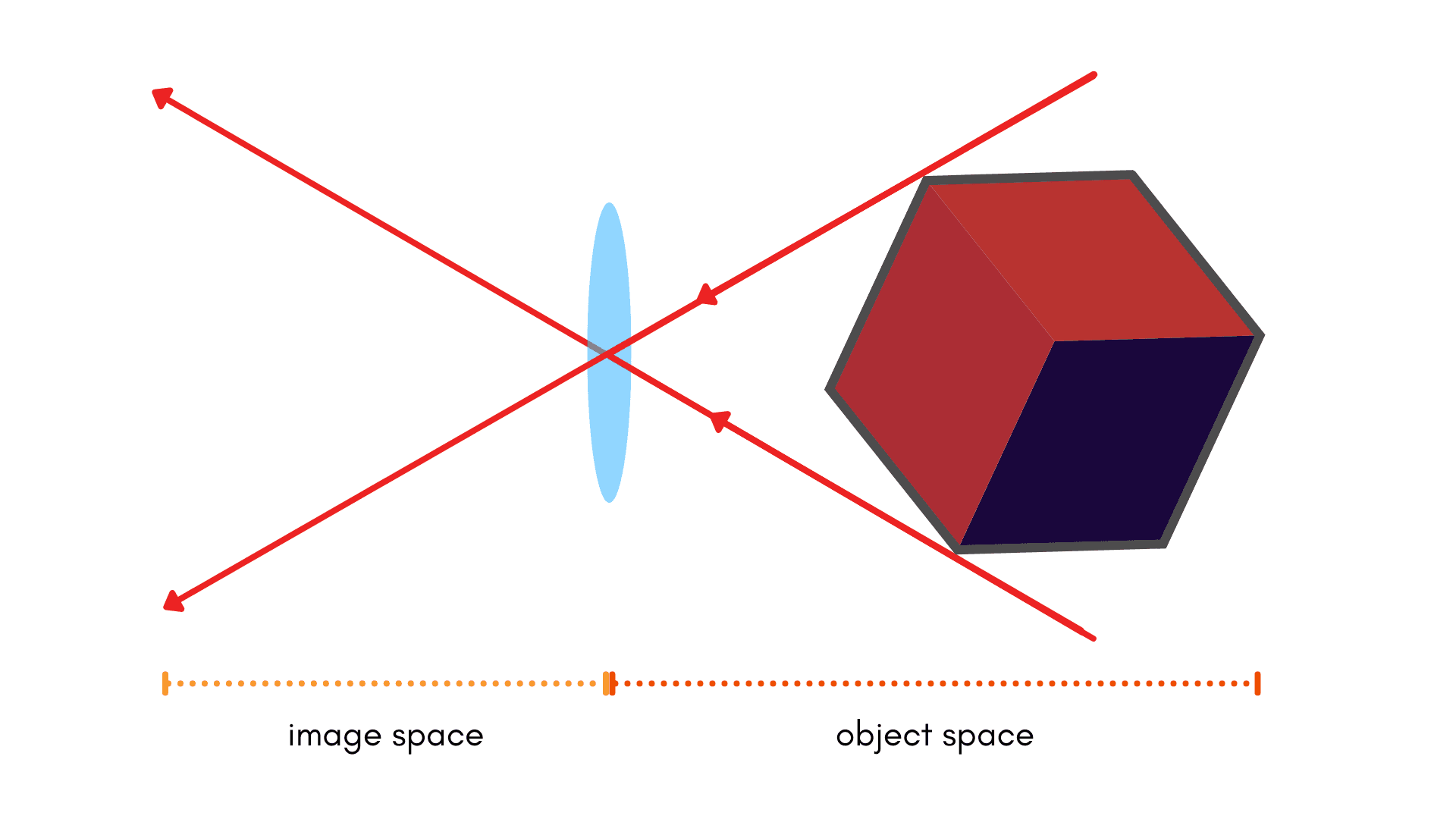
Here at Tangram Vision, we refer to our directly observed values as image measurements and our expected values as our object-space coordinates. We make direct measurements in image-space and relate that back to known quantities in object-space. Since we’re mainly discussing camera calibration here, we’ll be using “image-space measurements” and “object-space coordinates” for the rest of the post when discussing observed and expected values.
Forward and Inverse Distortion Models
The distinction between forward and inverse models may seem to some to have arisen from thin air; it’s not all that common in robotics or computer vision literature to make the distinction. Let’s start from first principles to help solidify what we mean.
Every model seeks to capture physical behavior, and camera models are no exception. When we optimize a camera model, we are deriving a mathematical way to describe the effect of the lens on the path of a ray of light.
The bad news: no model is perfect. There will always be systemic errors that result between our observations vs. our expected results. However, we can take one of two approaches to try and model these errors:
Applying a set of model parameters to our expected values in order to match directly observed quantities. We call this a forward model.
Applying a set of model parameters to our directly observed quantities in order to correct for systemic errors relative to our expected values. We call this an inverse model.
Did you catch the difference? It’s subtle, but vital.
What do forward models represent?
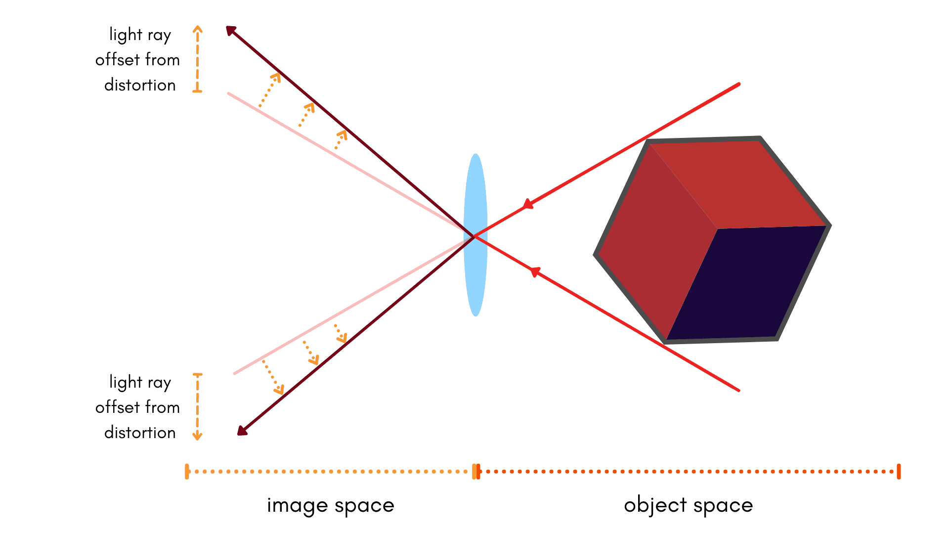
The forward distortion model takes the first approach to modeling systemic errors. Using our camera-specific terminology:
Applying a set of model parameters to our object-space coordinates in order to match our image-space measurements.
In this form, we apply distortion to camera rays made by projecting 3D points onto an image; we’re solving for the distortion, not the correction. In a very simplistic form, the forward model could be related as:
$$ \mathit{distorted} = \mathbf{f}(\mathit{ideal}) $$
Advantages of the forward model
Since after projecting a point into the image and applying the distortion model, we can directly relate the final “distorted” coordinate of the projection to measurements on the raw image itself.
The following equations represent how this looks in terms of the actual collinearity mathematics using a forward-Brown-Conrady model. Note that lowercase letter represent image-space quantities (e.g. \(x_i, y_i\)), whereas capital letters denote quantities measured in object-space (e.g. \(X, Y, Z\)).
First, we transform an object point in world space into the camera coordinate frame:
$$
\begin{bmatrix}X_c \\ Y_c \\ Z_c \end{bmatrix} = \Gamma_{\mathit{object}}^{camera} \cdot \begin{bmatrix} X_o \\ Y_o \\ Z_o \end{bmatrix}
$$
A term we call \(r_{f}\) describes a 3D point’s euclidean distance from a camera’s optical axis:
$$
r_{f} = \sqrt{X_c^2 + Y_c^2}
$$
We’ll use this term to model the effects of radial and tangential distortion on our light rays, and solve for where those distorted rays intersect the image plane:
$$
\begin{bmatrix} x_i \\ y_i \end{bmatrix} = f \cdot \begin{bmatrix} X_c / Z_c \\ Y_c / Z_c \end{bmatrix} + \begin{bmatrix} c_x \\ c_y \end{bmatrix} + \begin{bmatrix} X_c \left(k_1 r_f^2 + k_2r_f^4 + k_3r_f^6 \right) \\ Y_c \left(k_1 r_f^2 + k_2r_f^4 + k_3r_f^6\right) \end{bmatrix} + \begin{bmatrix} p_1 \left(r_f^2 + 2X_c^2\right) + 2 p_2 X_c Y_c\\ p_2 \left(r_f^2 + 2Y_c^2\right) + 2 p_1 X_c Y_c \end{bmatrix}
$$
Notice that all of our terms are derived from object-space coordinates \(X, Y, Z\). The only time we worry about the image at all is when the distorted pixel coordinates are spit out at the end! This is a classic forward model.
🔀 It’s worth mentioning here that OpenCV’s Brown-Conrady adaptation is a little different than what we’ve presented here. OpenCV presents a few crucial modifications to make working with their distortion profiles more user-friendly, and everything is done in normalized image coordinates. However, our explanation above still applies to the core of their model.
What do inverse models represent?
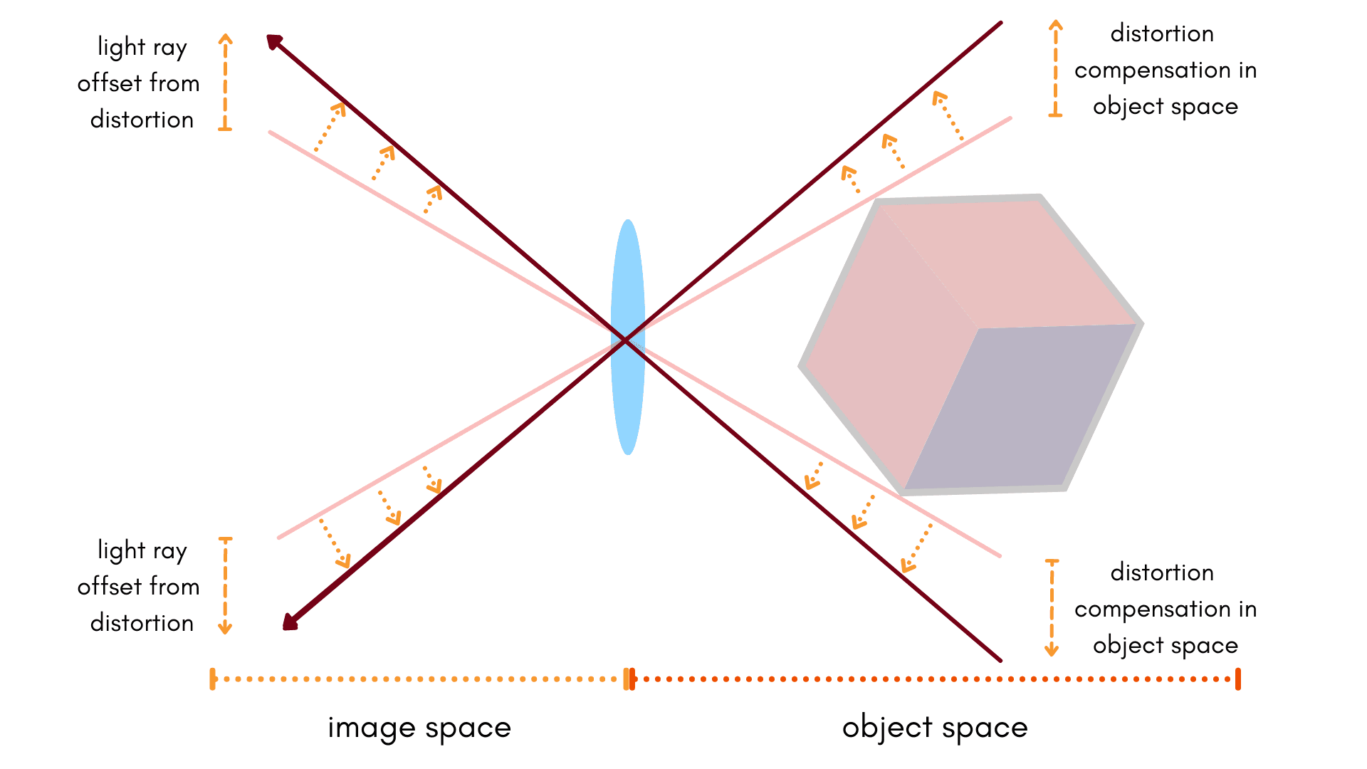
The inverse distortion model takes the second approach to modeling systemic errors. This means:
Applying a set of model parameters to our image-space measurements in order to correct for systemic errors relative to our object-space.
$$\mathit{ideal} = \mathbf{f}(\mathit{distorted})$$
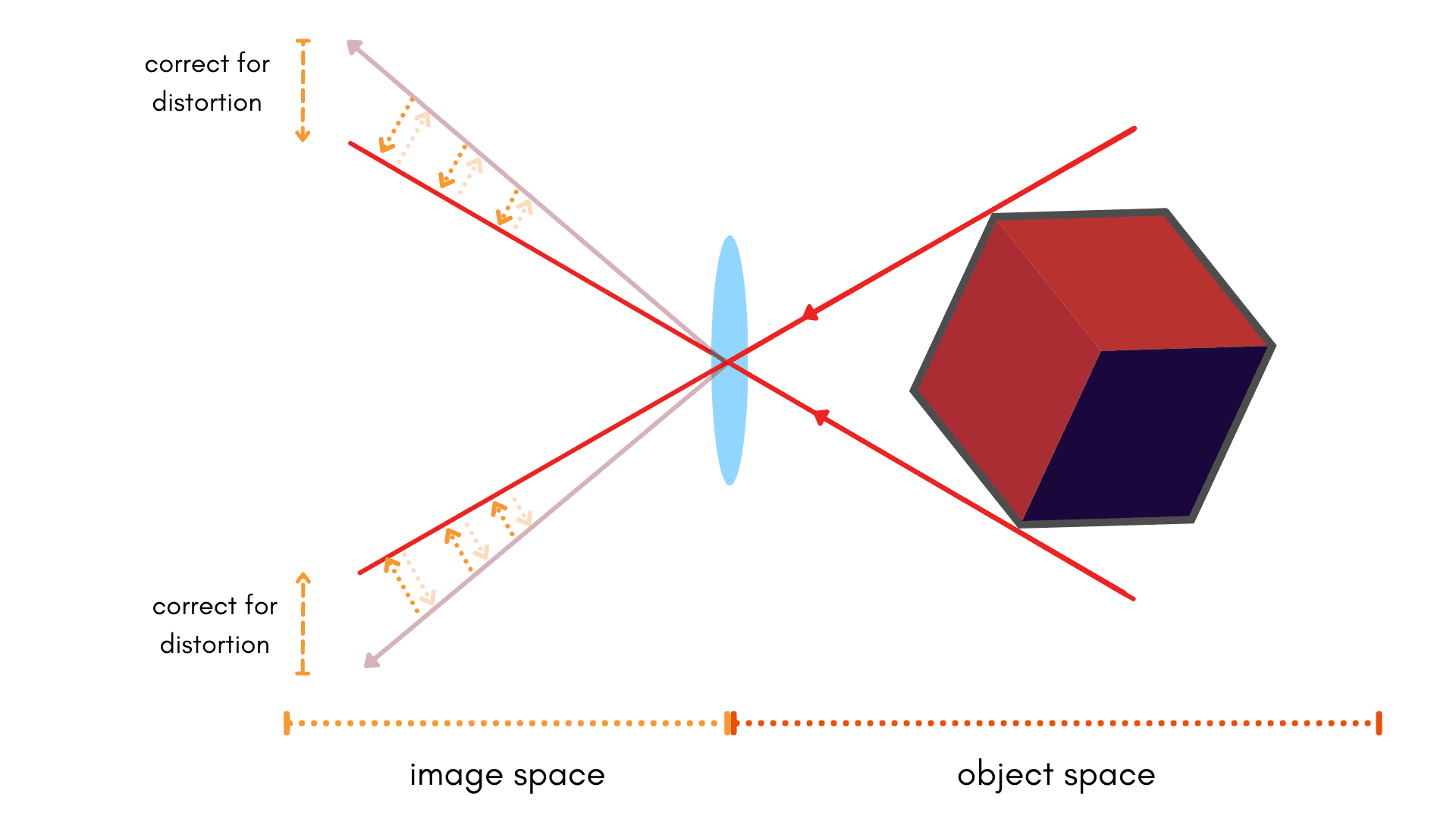
Advantages of the inverse model
In direct contrast to the forward model, the inverse model is useful if we’re starting with distorted points. It’s useful in situations when we want the pixel locations of points in the image after distortion is corrected — often referred to as a corrected or undistorted image.
The following equations represent how the inverse model looks in terms of the collinearity mathematics. Instead of using the forward Brown-Conrady model as adapted (after a fashion) by OpenCV, let’s use the inverse Brown-Conrady model instead. We’ll keep the same convention of capital letters for object-space entities and lowercase letters for image-space entities.
First, we transform an object point in world space into the camera coordinate frame (always):
$$\begin{bmatrix}X_c \\ Y_c \\ Z_c \end{bmatrix} = \Gamma_{\mathit{object}}^{camera} \cdot \begin{bmatrix} X_o \\ Y_o \\ Z_o \end{bmatrix}$$
But now our \(r\) term is different; we’re now calculating \(r_{i}\), the distance from the principal point of our camera in image space, relative to the principal point:
$$r_{i} = \sqrt{x_i^2 + y_i^2}$$
Using this \(r_{i}\) term, we can now model the correction of our distorted points.
$$\begin{bmatrix} x_i \\ y_i \end{bmatrix} = f \cdot \begin{bmatrix} X_c / Z_c \\ Y_c / Z_c \end{bmatrix} + \begin{bmatrix} x_i \left(k_1 r_i^2 + k_2 r_i^4 + k_3 r_i^6 \right) \\ y_i \left(k_1 r_i^2 + k_2 r_i^4 + k_3 r_i^6\right) \end{bmatrix} + \begin{bmatrix} p_1 \left(r_i^2 + 2 x_i^2\right) + 2 p_2 x_i y_i\\ p_2 \left(r_i^2 + 2 y_i^2\right) + 2 p_1 x_i y_i \end{bmatrix}$$
The inverse model therefore places our image-space coordinates on both sides of the equation!
Optimizing across a non-parametric equation like the inverse model is more difficult than optimizing a forward model; some of the cost functions are more difficult to implement. The benefit to the inverse approach is that, once calibrated, one could formulate the problem as follows:
$$\begin{bmatrix} x_i \\ y_i \end{bmatrix} - \begin{bmatrix} c_x \\ c_y \end{bmatrix} - \begin{bmatrix} u_i \left(k_1 r_i^2 + k_2 r_i^4 + k_3 r_i^6 \right) \\ v_i \left(k_1 r_i^2 + k_2 r_i^4 + k_3 r_i^6\right) \end{bmatrix} - \begin{bmatrix} p_1 \left(r_i^2 + 2 u_i^2\right) + 2 p_2 u_i v_i\\ p_2 \left(r_i^2 + 2 v_i^2\right) + 2 p_1 u_i v_i \end{bmatrix} = f \cdot \begin{bmatrix} X_c / Z_c \\ Y_c / Z_c \end{bmatrix}$$
Since all the parameters on the left only correspond to directly measured (i.e. distorted) coordinates in image-space, the left side of our equation doesn’t need to be optimized at all! This makes it simpler to use the calibration, since the distortion corrections do not rely or require knowledge of the pose of the camera.
Bridging the Gap
Attentive readers will notice that both the forward and inverse Brown-Conrady models have the same five distortion parameters:
$$k_{1}, k_{2}, k_{3}, p_{1}, p_{2}$$
However, these terms aren’t the same! One Brown-Conrady set of parameters operates on our expected values; the other operates on our observed values. One can’t just use the parameters interchangeably between forward and inverse models, despite them modeling the same distortion effects.
Converting between forward and inverse models
Instead, we can think about the operations that forward and inverse models perform:
Forward: f(object space) → distorted pixel space
Inverse: f(distorted pixel space) → corrected pixel space
If we consider object space points to be in homogeneous coordinates w.r.t. the camera, we can place the object space point in the image plane, which would essentially give us that object space point in corrected pixel space. Revisiting our comparison:
Forward: f(corrected pixel space) → distorted pixel space
Inverse: f(distorted pixel space) → corrected pixel space
Using this relationship, we find that the full inverse model can be used to optimize for the forward model, and vice versa. This is a lot of work, but knowing full sets of coefficients can be handy if one finds themselves locked into an API that only accepts a specific model.
❤️ …and it just gives us more opportunities to write non-linear optimizations! Everyone loves optimizations.
Using Look-Up Tables (LUTs)
Alternatively, one can use a lookup table. A “lookup table” refers to a matrix which transforms a distorted image to a corrected image (or vice-versa). It does this by assigning a shift in pixel space to every pixel in the image. It essentially saves the numerical effects of distortion into a matrix; instead of using the full distortion equations above to find a pixel, one can just save that answer once and “look up” what that effect would be later.
Since the model effects are calculated ahead of time, lookup tables allow one to avoid having to embed any esoteric math into a computer vision pipeline. One can now drag-and-drop different models into a program without fully implementing either forward- or inverse-specific logic. They are also incredibly useful when paired with GPUs, since an entire frame can be corrected or distorted in a single step.
💾 Tangram’s calibration software can output LUTs whenever needed. We have illustrated how to use LUT examples using native OpenCV functions in a code sample found here: https://gitlab.com/tangram-vision/oss/lut-examples.
Conclusion: What model should you pick?
As always, the model you pick is dependent on the use case. In the early days of Tangram, we chose inverse models for a few key reasons:
They transform distorted points into corrected points (which was the direction we wanted)
Their effects are additive in pixel space
Their formulation decouples model terms that are usually affected by projective compensation in most calibration pipelines
Using the calibration in a downstream perception pipeline is simplified, because the corrections from the inverse model do not depend on the pose of the camera at all.
Conversely, the forward model is most advantageous when:
Projecting 3D points from another modality (e.g. LiDAR) into the original, raw frame
You want to directly use software that supports only the forward model
💡 If you first “undistort” or correct your image with the inverse model, you can often use any forward model APIs with “zero” set distortion. Just remember that you aren’t working on the original, raw image!
As we’ve worked with more partners, we have adopted both inverse and forward models as the need arose. As long as one can understand the drawbacks and advantages, there’s no hard and fast requirement for using either style. Since we can use direct mappings such as look-up-tables (LUTs) or iterative solvers to switch back-and-forth between these models, the decision is more about picking one of two sides of the same coin.
…And does it matter?
In our experience, the single biggest factor in calibration quality isn’t the model; it’s the input data. Even a camera model perfect for one’s needs won’t produce a good calibration without the right training. This is why we start with the input process for every new calibration procedure we develop, no matter what camera model customers are using. Sometimes, better data makes it obvious that the model they were using was the wrong one! This is a best-case scenario: both process and outcome are improved in one fell swoop.


