IMU Preintegration Basics (Part 5 of 5)

So, you’ve purchased an IMU for a couple bucks and you’re not sure how to do anything useful with it? Your IMU state estimates seem to fly off beyond the horizon leaving you wondering what good is an IMU? You can’t seem to figure out how to read an IMU datasheet — I mean what is a \(\sqrt{Hz}\) anyway? It seems like you either have to hire an expert state-estimation engineer or pay thousands of dollars for a tactical-grade IMU?

Well, you’ve come to the right place. We are here to cure all your IMU woes and provide some insight into these confusing sensors. In this five part blog series, we’ll cover

• IMU sensing fundamentals
• Deterministic IMU error modeling
• Stochastic IMU error modeling
• The Allan Deviation and IMU error modeling
• IMU preintegration basics

If you’d like to be notified of when that next post drops, just follow us on LinkedIn, X, or subscribe to our newsletter. Don't have an IMU yet? Consider pre-ordering our upcoming HiFi depth sensor, for high-resolution 3D sensing...with a built-in IMU!

In previous posts in the series, we discussed the basic concepts around IMU operation and how to model the deterministic and stochastic errors in an IMU. If you’ve made it this far, congratulations! We are in the home stretch and are finally ready to process IMU data.

IMUs are rarely used as the only sensor on a robot. The pose inferred from integrating IMU data will always drift without bound unless corrected by some additional sensor, e.g. a camera, LiDAR, GPS, etc. Since there is so much flexibility in designing a robot and its navigation system, we are intentionally omitting any processing that must take place in order to use an IMU with an additional complementary sensor. However, be sure that in most robotics applications, you’ll want to use another sensor with your IMU.

With that caveat, let’s dive into IMU preintegration.

💡 This post is intended to be a high-level overview of IMU preintegration and the advantages it offers us. As such, we’ll only develop the minimal amount of mathematics needed to show why IMU preintegration is a cool idea.
For a full treatment of the subject the following sources are must reads:
‍
- Visual-Inertial-Aided Navigation for High-Dynamic Motion in Built Environments Without Initial Conditions
- On-Manifold Preintegration for Real-Time Visual-Inertial Odometry

IMU Motion Model

Our goal in this section is to introduce a motion model that connects the pose of the IMU to the outputs that an IMU provides. Before doing this, we will make the following assumptions:

• The scale and shear factors of the accelerometer and gyroscope are negligible and your IMU outputs scale and shear adjusted measurements.
• The \(g\)-sensitivity of the gyroscope is negligible.
• We have a way of obtaining a good estimate for the gyroscope and accelerometer biases.
• We know the local gravity vector \(g^i\) in the operating environment of our IMU and this local gravity vector does not change.

⚠️ If these assumptions are not valid for your IMU or operating conditions, you’ll have to develop your own preintegration and compensate for these errors correctly.

With these assumptions, the IMU kinematics are given by

                           \(\begin{aligned}
\dot{R}^i_b &= R_b^i
\left[\omega_{b/i}^b\right]_{\times} \\
\dot{p}_{b/i}^i &= v_{b/i}^i \\
\dot{v}_{b/i}^i &= a_{b/i}^i
\end{aligned}\)

Where

• \(R_b^i\) is the “body” frame of the IMU expressed in the inertial frame
• \(\omega_{b/i}^b\) is the angular velocity of the IMU with respect to the inertial frame expressed in the body frame of the IMU
• \(\left[\ \cdot\ \right]_{\times}\) is an operator to take the cross product matrix
• \(p^i_{b/i}\) is the position of the IMU with respect to the inertial frame expressed in the inertial frame
• \(v_{b/i}^i\) is the velocity of the IMU with respect to the inertial frame expressed in the inertial frame
• \(a_{b/i}^i\)  is the acceleration of the IMU with respect to the inertial frame expressed in the inertial frame here

The inertial frame that you choose will depend on your application and your ability to provide global state information (perhaps using GPS). These kinematics are not in terms of our measured variables. Recall our original simplified measurement model given by

                           \(\begin{aligned}
\tilde{\omega}_{g/i}^g(t) &=
\omega_{g/i}^g(t) + b_g^g(t) +
\eta^g_g(t) \\
f^a(t) &=
a_{a/i}^a(t) + b_a^a(t) - R^a_i(t)
g^i + \eta^a_a(t)
\end{aligned}\)

Ignoring the noise terms and solving for our state variables, we can create navigation equations based on the IMU measurements

                           \(\begin{aligned}
\dot{R}^i_b &= R_b^i
\left[\tilde{\omega}_{b/i}^b -
b^b_g\right]_{\times} \\
\dot{p}_{b/i}^i &= v_{b/i}^i \\
\dot{v}_{b/i}^i &= R^i_b(f^b - b^b_a) + g^i
\end{aligned}\)

Creating kinematic equations that are driven directly from IMU inputs is commonly known as IMU mechanization. In discrete time, these equations can be formulated as

                           \(\begin{aligned}
{R}^i_b(t + \Delta t) &= R_b^i(t)
\text{Exp}\left(\Delta t\left[\tilde{\omega}_{b/i}^b - b^b_g\right]{\times}\right) \\
{p}_{b/i}^i(t + \Delta t) &= p_{b/i}^i(t) + \Delta t v_{b/i}^i(t) + \frac{1}{2}\Delta t^2 g^i + \frac{1}{2}\Delta t^2 R^i_b(t)\left(f^b - b^b_a\right) \\
v_{b/i}^i(t + \Delta t) &= v_{b/i}^i(t) + \Delta t g^i+ \Delta t R^i_b(t)\left(f^b - b^b_a \right)\end{aligned}\)

⚠️ If this discretization for rotation looks surprising or unfamiliar, we’ll refer the interested reader to an excellent tutorial on lie theory. Full understanding of the discretization here is not necessary to grasp the benefits of IMU preintegration.

Naïvely, we could use this as our integration model. In short, we take our raw IMU samples, transform them into the inertial frame and then we fold them into our state estimate. When we update our states, we should also update the covariance of our states and ensure we combine the covariance on the IMU measurements with the covariance of the state correctly. Hopefully, we won’t get stuck in a bad state estimate due to a particularly noisy IMU sample. In a few moments, our estimates don’t look very good and the measurement updates from our complementary sensor are making our navigation estimate jitter.

As you can see, there are many downsides to the naive application of this approach. This leaves us with the question: is there a better way to handle IMU measurements?

IMU Preintegration

One key insight behind IMU preintegration is the realization that our inertial frame is somewhat arbitrary. As long as we know the gravity vector \(g^i\), we could perform the integration in any frame. For a moment, let’s just pretend that our previous keyframe aligns with the origin of the inertial frame and is not moving. Then we would have a discretized motion model of

                           \(\begin{aligned}{R}^i_b(t + \Delta t) &= \text{Exp}\left(\Delta t\left[\tilde{\omega}_{b/i}^b - b^b_g\right]_{\times}\right) \\
{p}_{b/i}^i(t + \Delta t) &= \frac{1}{2}\Delta t^2 g^i + \frac{1}{2}\Delta t^2 \left(f^b - b^b_a\right) \\
v_{b/i}^i(t + \Delta t) &= \Delta t g^i+ \Delta t\left(f^b - b^b_a \right)\end{aligned}\)

This already looks a lot simpler! Furthermore, let’s pretend that the output on the accelerometer was a real acceleration and not simply a specific force measurement. In other words, let’s pretend that we somehow have already performed gravity compensation on the IMU measurement \(f^b\). While we are at it, let’s rename this value and call it the “local increment” of the previous keyframe \((\Delta R, \Delta p, \Delta v).\) Now we have a discretized motion model of

                           \(\begin{aligned}\Delta R &= \text{Exp}\left(\Delta t\left[\tilde{\omega}_{b/i}^b - b^b_g\right]{\times}\right) \\
\Delta p &=  \frac{1}{2}\Delta t^2 \left(f^b - b^b_a\right) \\
\Delta v &= \Delta t\left(f^b - b^b_a \right)\end{aligned}\)

If we look close, we’ll realize that this value only depends on the previous keyframe semantically but does not use the pose or velocity of the keyframe in any mathematical way. Furthermore, since we are ignoring gravity, we can continue to accumulate measurements in this local increment.

Local Increment Computation

Computing the local increment is actually a fairly simple task. In our opinion, this is best presented in algorithmic form (if you want to see all the mathematical details, we’ll refer you to the previously mentioned papers).

First, we start by initializing some variables

                           \(\begin{aligned}\Delta R &\gets I \\ \Delta p &\gets 0 \\ \Delta v &\gets 0 \\ \Delta t &\gets 0 \\ t_{prev} &\gets t_{first} \end{aligned}\)

Where

• \(t_{prev}\) is the timestamp of previous sample
• \(t_{first}\) is the timestamp of the start of the preintegration
• \(\Delta R\) is the rotation increment since the previous keyframe
• \(\Delta p\) is the positional increment since the previous keyframe
• \(\Delta v\) is the velocity increment since the previous keyframe

Then we simply accumulate the IMU measurement terms into this local increment as we receive them. Given the IMU bias we simply perform the following steps upon receiving a new IMU measurement

                           \(\begin{aligned}\delta t &\gets (t_{samp} - t_{prev}) \\ \delta R &\gets \text{Exp} \left(\delta t\left[\tilde{\omega}_{b/i}^b - b^b_g\right]_{\times}\right)\\ \delta p &\gets \frac{\delta t^2}{2}(f^b - b^b_a) \\ \delta v &\gets \delta t(f^b - b^b_a) \\ \Delta t &\gets \Delta t + \delta t \\ \Delta p &\gets \Delta p + \Delta v \delta t + \Delta R \delta p \\ \Delta v &\gets \Delta v + \Delta R \delta v \\ \Delta R &\gets \Delta R \delta R \\ t_{prev} &\gets t_{samp}\end{aligned}\)

Where

• \(t_{samp}\)  is the timestamp of the IMU sample
• \(\delta R\) is the induced local rotation increment from the latest IMU sample
• \(\delta v\) is the induced local velocity increment from the latest IMU sample
• \(\delta p\) is the induced local position increment from the latest IMU sample and local velocity increment

This is the entirety of the local increment calculation and the algorithm shows this quite simply: take the rates, scale them by time and accumulate them into the local increment. For convenience, integration jacobians are also typically calculated during the preintegration. You can find more details regarding the jacobian calculations in the referenced papers.

⚠️ Of particular note is the order in which we update our local increment states. The algorithm presented here is a zero-order hold integration and is an exact integration under a zero-order hold assumption. In reality, the accelerometer data is a sample during the preintegration window and the actual acceleration is changing during this window. To compensate for this error induced by sampling, one can perform higher-order integrations provided that proper coning and sculling compensations are applied.
‍
Any error in the integration process is naturally called “integration error.” Integration error can be handled by adding an integration error covariance term during adjustment or filtering. In practice, integration error is dwarfed by other deterministic and stochastic sources of error and is often left unmodeled.

Where is gravity?

In the previous sections, we’ve explicitly ignored gravity because the gravity terms are inextricably tied to our choice of inertial frame. In other words, we cannot integrate the terms associated with gravity until we know the keyframe’s pose with respect to the inertial frame. Furthermore, if we added the gravity terms to our local increment, we would have to transform them into the keyframe and then recalculate them upon every adjustment of the keyframe.

By momentarily ignoring the gravity terms, we can transform a high-rate IMU data stream into a low-rate measurement stream that is approximately synchronized to a complementary sensor’s data. We do, however, have to account for gravity eventually. Rewriting our original discretization in terms of the preintegrated variables, we get:

                           \(\begin{aligned}{R}^i_b(t + \Delta t) &= R_b^i(t) \Delta R \\ {p}_{b/i}^i(t + \Delta t) &= p_{b/i}^i(t) + \Delta t v_{b/i}^i(t) + \frac{1}{2}\Delta t^2g^i + R^i_b(t)\Delta p \\ v_{b/i}^i(t + \Delta t) &= v_{b/i}^i(t) + \Delta t g^i + R^i_b(t)\Delta v\end{aligned}\)

where \(\Delta t\) is the time between keyframes. These equations can easily be manipulated to create the parametric measurement model

                           \(\begin{aligned}\Delta R &= R^i_b(t)^\top {R}^i_b(t + \Delta t) \\ \Delta p &= R^i_b(t)^{\top} \left({p}_{b/i}^i(t + \Delta t) - p_{b/i}^i(t) - \Delta t v_{b/i}^i(t) - \frac{1}{2}\Delta t^2g^i\right) \\ \Delta v &= R^i_b(t)^{\top} \left(v_{b/i}^i(t + \Delta t) - v_{b/i}^i(t) - \Delta t g^i\right).\end{aligned}\)

We’ve now computed a local increment and formulated its usage in a measurement model, completing our preintegration. In fact, this is why we call it preintegration because we integrate the IMU measurements prior to using the local increment in an estimation.

Physical Interpretation of Preintegration

The local increment (preintegrated measurement) has an interesting physical interpretation. Since gravitational specific force can be interpreted as acceleration relative to a free-falling body, the local increment can be interpreted as the change in pose as compared to the previous free-falling keyframe. In other words, from the previous keyframe’s point of view, the local increment is accelerating upward at \(g\). The addition of the gravity terms is simply an adjustment to compensate for the nature of the “apparent free-falling” keyframe.

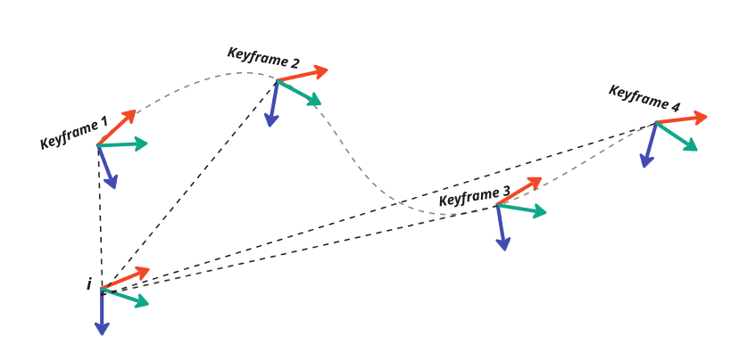
We can also think about this graphically. Without preintegration, we express everything in a global context, transforming all measurements to an inertial frame before using them. This is shown graphically in the diagram below.

With preintegration, we express accumulated IMU measurements local to their own frame of reference. You can see this is the diagram below.

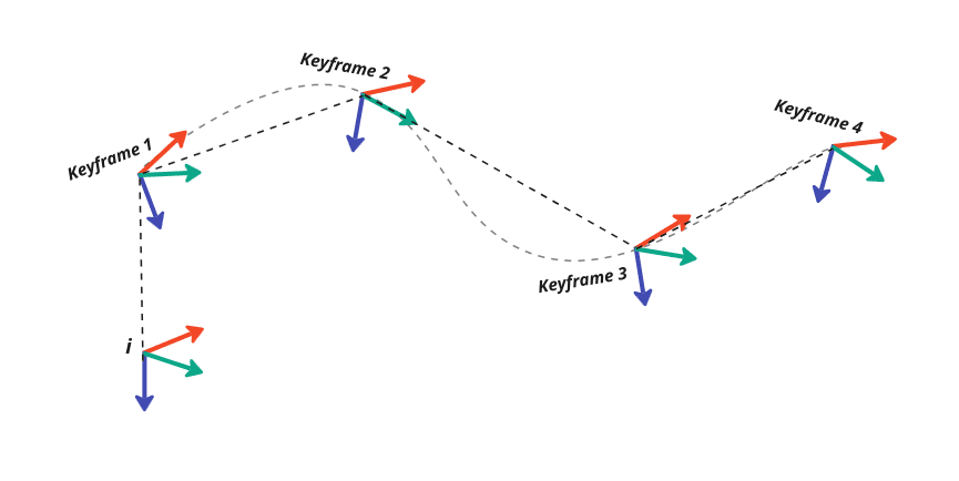
In both cases, we are trying to estimate the same keyframes and the same path. We are simply changing how we represent and process the IMU measurements.

Benefits of Preintegration

At this point, you may be saying “So what? All we’ve done is shuffle some terms around” and honestly, you’re right. All we’ve done is change how we think about the problem and change the sequence in which we process IMU measurements: preintegrating before estimating a navigation state. However, there are actually some notable benefits to the preintegration approach.

• Since we don’t incorporate our raw IMU samples into the navigation estimate, we save compute cycles on expensive operations like state covariance propagation. We can perform the more expensive operations at a lower rate. This also helps in preventing addition of too many keyframes to an adjustment.
• Using preintegrated measurements allows us to craft algorithms that are less sensitive to the frame rate and syntonization of our complementary sensors. We can simply integrate until a measurement from a complementary sensor arrives. In effect, this means that preintegration methods are robust to dropped frames.
• When comparing to other types of measurements, we now treat measurements in the same way mathematically. There is no special case of “if this is an IMU measurement,” use it to propagate the estimate, otherwise use it to correct the estimate. All measurements are now used to correct state estimates.
• Since preintegrated values are treated as measurements and not inputs to a mechanized motion model, a long preintegration period won’t cause the navigation covariance to blow up. Adjustment or filtering techniques relying on preintegration will simply weigh the relative information from the IMU vs the complementary sensor. Thus, using preintegration means we don’t commit to a bad intermediate state estimate and linearization simply because we got a couple of noisy IMU samples. This correct weighting ultimately makes the navigation estimate more accurate and less noisy.
• The same preintegration engine can be used in either a filtering or an adjustment context. This obviously has benefits for creating generic algorithms that can be adapted to the compute restrictions of your device.
• If preintegration is used in an adjustment context, out-of-sequence or late measurements can be handled without requiring reintegration of the navigation state.

What about the Bias?

The entire preintegration algorithm hinges on one big assumption: we have a good estimate of the IMU bias. Obtaining an accurate bias estimate of the IMU independent of the navigation estimate is a tough ask and without a good bias estimate, the preintegration is not accurate. For this reason, state estimation engineers will include the IMU bias into the estimated state. However, when the bias is included in the state, our preintegration is no longer decoupled from the state since the bias is needed to compute the preintegration. In other words, our local increment depends on our estimate of the bias.

We fix this problem by applying a first-order correction to our preintegrated measurements. Explicitly, whenever we compute a bias update \(\delta b^b_g\) and \(\delta b_a^b\) (whether in a filtering or optimization context), we will correct our preintegrated measurements with

                           \(\begin{aligned}\Delta R &\gets \Delta R \text{Exp}\left(\frac{\partial \Delta R}{\partial b^b_g} \delta b^b_g\right) \\
\Delta p &\gets \Delta p + \frac{\partial \Delta p}{\partial b^b_g} \delta b^b_g + \frac{\partial \Delta p}{\partial b^b_a}
\delta b^b_a \\ \Delta v &\gets \Delta v + \frac{\partial \Delta v}{\partial b^b_g} \delta b^b_g + \frac{\partial \Delta v}{\partial b^b_a} \delta b^b_a \end{aligned}\)

Now, we can continue use these corrected preintegrated measurements in a filtering or adjustment context.

⚠️ Strictly speaking, the first-order correction is not mathematically correct. The correction performs a similar function to the residual jacobian with respect to the observations that would be used in a total least squares adjustment, but the first-order correction lacks the proper residual computation and weighting for correctness.

However, the error induced by a first-order correction is minor as shown in the previously referenced papers. As such, it is common practice to use this correction despite being mathematically incorrect.

Wrapping Up

This concludes our high-level overview of IMU preintegration. There are many things that we didn’t cover such as:

• How to characterize the uncertainty of preintegrated measurements
• How to use the preintegrated values in an optimization or filtering context
• How to choose a preintegration method (here we presented a zero-order hold preintegration, but some circumstances may warrant higher-order integration methods)
• Should raw IMU samples ever be reintegrated if the IMU bias drifts?
• How to obtain a good initial bias estimate

Finally, on a related note, our latest MetriCal multimodal calibration software release now supports IMU calibration. In fact, it was the process of building this latest MetriCal release that inspired me to write this 5-part series on IMUs! If you'd like to try it with your own robot or autonomous vehicle, reach out to request a trial.

I hope these guides are useful as you develop your robot or AV’s sensor systems. If you’d like to be notified of when our next blog post drops, just follow us on LinkedIn, X, or subscribe to our newsletter.