This article is a continuation of Plane Fitting, Part 1 and builds heavily on our Camera Modeling articles. If you haven’t done so, go back and check those articles out.

Want to follow along at home? We have a working example with source code and results in this Colab notebook.

—

Intro

In the last article, we looked at plane fitting as a parametric least squares problem. We encountered an issue using the most straightforward, obvious cost for plane fitting:

$$ \underset{\hat{n},d}{\text{argmin}}\sum_{i}\left\lVert \hat{n}^Tx_i-d \right\rVert_{2}^{2} $$

Since the normal must be a unit vector, this is a constrained optimization problem. The space of 3D unit-vectors $S^2$ is a smooth manifold (Dyna and Tillo would agree), but it is not a Lie group, so the techniques we use to optimize manifolds that are Lie groups (rotations, poses, similarities etc.) don’t apply directly. In the last article we identified a trick to use a subset of 3D rotations (which are a Lie group). In this article, we’ll talk about optimizing on-manifold more generally, while focusing on $S^2$.

Motivation

But first: why this is even worth writing about?

If you’re like me, you found yourself in this corner of the world of mathematics out of a direct, concrete necessity. You might have started in on some estimation problem in robotics or computer vision and found yourself trying to optimize some constrained quantity like a rotation or isometry. After a bit of research, you come across Lie groups or some similar representation and start plugging in equations.

However, in the world of manifolds, Lie groups are an exception. They possess certain properties that make them easier to work with than other manifolds which aren’t Lie groups. In the fields of robotics and 3D computer vision, there’s a special emphasis on Lie groups because many, if not all, of the manifold quantities (rotations, isometries, etc.) one might be initially interested in are in fact Lie groups. The emphasis is strong enough that it's perhaps common for those starting out in these fields to jump past not only smooth manifolds, but even Lie groups more generally and just focus on e.g. rotations / SO(3) — learning only what’s needed to start optimizing.

This represents a reversal in how things might be framed in a first-principles treatment of these concepts from the field of differential geometry. Aside from giving us a path forward in optimizing over $S^2$, moving beyond just Lie groups meant (for me at least) a useful broadening of understanding of manfold optimization fundamentals.

Manifold Optimization Fundamentals

Not All Manifolds Are Lie Groups

As explained in our Camera Modeling blog post (”The Asymmetric Unit Sphere”) Lie groups possess a property of continuous symmetry of their tangent spaces. Put differently, the tangent space is everywhere isomorphic to itself. This means we can use the tangent space at the identity of the group as the tangent space for every member of the group.

This also means we can map between points on the manifold and points in the tangent space at the identity, in such a way that elements of the tangent space can represent the values on the manifold. Thus, we can store tangent space coordinates in place of manifold points. For example, we can store a 6 degree-of-freedom transformation as a set of 6 tangent space coordinates instead of a 3x4 matrix / Quaternion + translation etc., and still be able to recover the transform. This isn’t necessarily possible when the manifold in question is not a Lie group, because the tangent space is going to differ locally.

Varying Tangent Spaces in Manifolds

Let’s dissect how we map elements on the manifold to and from tangents space elements. Recall the two manifold operations: “retract” which map an element of the tangent space at point p on the manifold onto the manifold and “local” which maps a point p1 on the manifold to the tangent space defined at another point p on the manifold. Note that retract and local can be any function which smoothly performs these mappings and thus a manifold doesn’t necessarily have one unique retract or local function.

$$ \begin{align} \text{Retract}_{p}(v) &: \mathcal{T}_p\mathcal{M} \mapsto \mathcal{M} \\ \text{Local}_{p}(p_1) &: \mathcal{M} \times \mathcal{M} \mapsto \mathcal{T}_p\mathcal{M} \end{align} $$

For general manifolds, the retract and local operations must be parameterized at a given point. In other words, tangent space varies from point to point; the tangent space coordinates (v) don’t have meaning if they’re not paired with a point on the manifold.

Lie Groups: Exceptions To The Rule

However, this is not true for Lie groups. For these, the tangent space at p is isomorphic everywhere. This fact, and the group operation that all Lie groups have by definition, gives the retraction and local operations a more specific form.

$$ \begin{align} \text{Retract}_p(v) &= p \cdot \text{exp}(v) \\ \text{Local}_p(p_1) &= \text{log}(p^{-1} \cdot p_1) \end{align} $$

The exponential and logarithm maps for Lie groups map manifold elements from the tangent space at the identity and to the tangent space at the identity respectively.

Note that the geodesic (the result of the exponential map, or similarly the on-manifold difference between p1 and p) isn’t parameterized by p. We can interpret the retract operation as shifting the geodesic such that it represents an otherwise independent perturbation to one local to p.

Some of the ordering of group operations and interpretation of the retraction as a local-rather-than-global perturbation follows from a right-handed convention and that there’s also a left-handed one.

Optimizing on the Manifold

There are numerous resources and techniques available for optimizing on a manifold. In the context of 3D computer vision, we often find ourselves writing non-linear, unconstrained, least squares problems like so:

$$ \underset{x}{\text{argmin}}||r(x)||^{2} $$

We solve this using iterative Gauss-Newton-like algorithms whicl approximate the residual function using the first order Taylor expansion:

$$ r_i(x+\Delta x)\approx r_i+J_i(x)\Delta x $$

And then each iteration produces a set of normal functions and updates to the parameter space:

$$ \begin{align} r_i + J_i(x)\Delta x &= 0 \\ J_i(x)\Delta x &= -r_i \\ \Delta x &= (J^T J)^{-1}J^T r \\ x_{i+1} &= x_i + \Delta x \end{align} $$

We’ll consider optimizing in this context.

Addition Through Retraction

When working with the standard version of this algorithm. where parameters live in a familiar vector space like $\mathbb{R}^n$, the tangent space to the parameters is that same vector space. In this case, adding a parameter and a parameter update in the tangent space is perfectly valid.

However, to adapt Gauss-Newton for manifolds (whether Lie groups or not), we must recognize that the updates $\Delta x$ lie in the tangent space of the parameters. This follows from linearization. Adding elements of the parameter space and tangent space may not be defined, and even when defined, may not produce an element of the parameter space.

Our goal is to optimize a parameter while staying on the manifold (e.g., to maintain constraints like rotation validity or position on a sphere). Addition, even when defined, may move the parameter off the manifold entirely. For the unit sphere in 3D ($S^2$), for instance, adding a value on the manifold (a point on the sphere) to a point in the tangent space pulls that point off the sphere. No good! So what does “addition” mean for our manifold? How do we stay on-manifold for the duration of our optimization?

The retract operation is our way forward. It will help us out in a few ways. First and foremost, retract is compatible with updating a parameter: in other words, It takes a parameter value and a tangent space value and produces a new parameter value. More importantly, though, the retraction produces a new parameter value that’s coherent with the tangent space value and the current parameter value. In essence, retraction maps changes in the tangent space to changes in the parameter.

Adapting Gauss-Newton for the Manifold

Normal Equations

Let’s use this knowledge to form our on-manifold version of Gauss-Newton:

$$ \begin{align} r_i(x \oplus \Delta x) &\approx r_i + J_i(x)\Delta x \\ J &= \frac{\partial r(x \oplus \Delta x)}{\partial \Delta x} \end{align} $$

This may look almost identical to our original formulation, but it differs in a few important ways:

• $\Delta x$ is more explicitly a set of local tangent space coordinates

• Retraction $\oplus$ is used in place of addition

• The Jacobian is computed using a compatible definition of a derivative which uses retract and local operations (see Micro Lie Theory (41a) for a similar, but Lie group specific version)

Parameter Update

The parameter update solve also may look the same, but we update the parameter like so:

$$ x_{i+1} = x_i \oplus \Delta x $$

While this formulation may seem specific to manifolds, it perfectly handles the conventional vector space case. $\mathbb{R}^n$ is trivially a manifold, after all, and with addition and subtraction used as the retract and local operations, we get back to our original formulation.

Jacobians

The only remaining discrepancy is the Jacobian. In vector-space GN, the jacobian is of the residual function at parameter vector $x$ with respect to $x$, which differs from what we have a above.

$$ \begin{align} J_{\mathbb{R}^n} &= \frac{\partial r(x)}{\partial x} \\ J_{\text{manifold}} &= \frac{\partial r(x \oplus \Delta x)}{\partial \Delta x} \end{align} $$

Let’s apply the chain rule to break down the on-manifold jacobian:

$$ J_{manifold}=\frac{\partial{r(x\oplus \Delta x)}}{\partial{(x\oplus \Delta x)}} \cdot \frac{\partial{x\oplus \Delta x}}{\partial{(\Delta x)}} $$

The first term is our familiar Jacobian from vector-space GN (sub $x'=x\oplus\Delta x$ if it’s not clear). The second term is the Jacobian of our retraction, which for addition over vectors, simply becomes the identity. Thus the manifold version of GN can completely encompass the vector one. This is useful: we can mix manifold and non-manifold parameters into one vector and use the same algorithm. We’ll do so later when we get back to our plane fitting example.

So: all we need to optimize on a manifold is a retraction and the relevant Jacobians. If the manifold in question is a Lie group we can use the retract method from the previous section. However, sadly for us, $S^2$ is not a Lie group; we’ll have to come up with something else.

Optimizing over $S^2$

2D - 3D tangent space mapping for $S^2$

Before we can even discuss the retract operation for $S^2$, there’s the matter of coming up with a minimal parameterization of the tangent space at a point p.

The tangent space of a point on a 3D sphere is a plane. Elements of this tangent space are thus 3D vectors, but with the constraint that they live on that plane. Given the point on the sphere, and thus its tangent space (i.e. the plane tangent to the sphere at that point), an element of the tangent space really only has two degrees of freedom: the in-plane coordinates.

To optimize in the tangent space while avoiding constrained optimization, we need to avoid parameterizing tangent space elements as 3D vectors with constraints. Instead, we parameterize elements of the tangent space as a 2D vector and provide a mapping from that 2D vector to an actual 3D element of the tangent space of the sphere. With this mapping, any 2D vector can be related to an element of the tangent space at a point.

The mapping is somewhat arbitrary. You might, for example, try to relate the X and Y coordinates of the 2D tangent space to the X and Y coordinates in 3D so that the 2D tangent space coordinates and the resulting 3D tangent space vectors are aligned. It's not a bad thought, but that strategy is doomed to fail on its own. Because of the 3D sphere's inherent properties (discussed previously in our Camera Modeling blog post), any single mapping will have a degeneracy somewhere. In fact, this relates to why the 3D sphere is not a Lie group. If we tried to align the X and Y axes of the 2D plane with the X and Y axes in 3D, we'd have a degeneracy at the "poles" of the sphere—points on the Z axis would have an entire family of 2D-3D tangent space mappings that satisfy the alignment criterion.

The solution is to make the mapping piecewise. This is where it gets arbitrary: any approach that is consistent, unique and avoids numerical issues should work. GTSAM has a strategy which partitions the sphere into 3 areas; however, to hammer home the arbitrary nature of the approach, here’s a different one I came up with:

1. Pick a starting reference axis. If the point on the sphere isn’t too close to the +/- Z axis, then use the Z axis; otherwise use the X axis.

2. Use the cross product to find a vector perpendicular to the vector representing the point on the sphere and the reference axis. The cross product is degenerate if the two vectors are parallel, which is why we specifically avoid that case in step 1. Normalize the result, forming a unit vector.

3. Use the cross product again to find a vector perpendicular to the sphere point vector and the vector found in step 2. Normalize the result, forming a unit vector.

4. Stack the results of step 2 and 3 to form a $3\times2$ matrix which maps 2D tangent space coordinates to 3D. We’ll call this $M_{\text{basis}}$

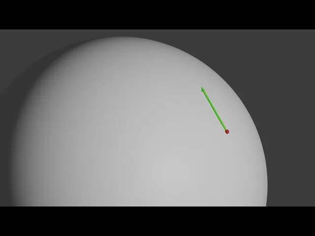
It’s important to emphasize that this mapping is different at each point on the sphere. You can see this visually in the graphic below.

This illustration shows how a 2D tangent space vector can map to different 3D tangent space vectors at various points on the sphere.

Retract and the Exponential Map

Now that we’ve got a 3D tangent vector, we need a retract operation, which will take the form of the exponential map. The exponential map relates a tangent vector to a “shortest” path on the manifold, “shortest” here being measured according to the constraints of the manifold. In general, this path is called the geodesic.

Depending on the manifold, the exponential map can difficult to compute; there are simpler retractions which only approximate the geodesic. Fortunately for those in robotics and perception, the manifolds we work with day-to-day often have closed form solutions. Our luck is even better given our sphere example: the shortest path between two points is just a segment of one of the sphere’s great circles. We’ll use this concept to come up with the exponential map.

Solving the Geodesic

Since a great circle on a 3D sphere lies in a 2D plane, we can think of our geodesic as the path traced out by rotating a point on the unit circle in that plane.

Let’s arbitrarily say we want to perform our rotation in the XY plane. To do so, we have to compute a rotation which brings our geodesic into the XY plane. What rotation would provide this mapping? Consider solving the following equation for $R_{\text{to-xy}}$, where $p, \hat t, \hat u$ are the point on the sphere, the normalized tangent vector and some third orthonormal vector respectively:

$$ R_{\text{to-xy}} \begin{bmatrix} \vert &\vert&\vert \\ p & \hat{t} & \hat u \\ \vert & \vert & \vert \end{bmatrix} = I $$

Solving this will align $p, \hat t, \hat u$ with the X, Y, and Z vectors (i.e. the columns of the identity matrix) respectively. This will place $p, \hat t$ in the XY plane.

Since all vectors involved are orthonormal, the solution is straightforward:

$$ R_{\text{to-xy}} = \begin{bmatrix} p^T \\ \hat{t}^T \\ \hat{u}^T \end{bmatrix} $$

Now that we’re in the XY plane, our geodesic is like a 2D rotation embedded in 3D. Thus, our exponential map rotation in the XY plane is formed by embedding a 2D rotation matrix into a 3D matrix. We just need to calculate the angle $\theta$ for our rotation.

The arc length of a geodesic is $arc = r\theta$. This is a unit sphere, so $r=1$. The exponential map “wraps” the tangent vector onto the manifold such that the arc length equals the length of $t$: $arc=\|t\|$, thus $\theta = \|t\|$

$$ R_{\text{xy-exp}}=\begin{bmatrix} \cos{\theta} & -\sin{\theta} & 0 \\ \sin{\theta} & \cos{\theta} & 0 \\ 0 & 0 & 1 \end{bmatrix} $$

The rotation which applies the exponential map is formed by first rotating the point into the XY plane, rotating in the XY plane, and then rotating back to our original coordinate frame.

$$ R_{\text{exp}}=R_{\text{to-xy}}^TR_{\text{xy-exp}}R_{\text{to-xy}} $$

So finally, the exponential map as parameterized by $p, t$ is:

$$ \text{exp}(p, t)=R_{\text{to-xy}}^TR_{\text{xy-exp}}R_{\text{to-xy}}p $$

$$ \text{exp}(p, t)=\begin{bmatrix} p & \hat{t} & \hat{u} \end{bmatrix}\begin{bmatrix} \cos{\|t\|} & -\sin{\|t\|} & 0 \\ \sin{\|t\|} & \cos{\|t\|} & 0 \\ 0 & 0 & 1 \end{bmatrix}\begin{bmatrix} p^T \\ \hat{t}^T \\ \hat{u}^T \end{bmatrix} p $$

$$ \text{exp}(p, t)=\begin{bmatrix} p & \hat{t} & \hat{u} \end{bmatrix}\begin{bmatrix} \cos{\|t\|} & -\sin{\|t\|} & 0 \\ \sin{\|t\|} & \cos{\|t\|} & 0 \\ 0 & 0 & 1 \end{bmatrix}\begin{bmatrix} 1 \\ 0 \\ 0 \end{bmatrix} $$

$$ \text{exp}(p, t)=\begin{bmatrix} p & \hat{t} & \hat{u} \end{bmatrix}\begin{bmatrix} \cos{\|t\|} \\ \sin{\|t\|} \\ 0 \end{bmatrix} $$

$$ \text{exp}(p, t)=\cos({\|t\|})p + \sin(\|t\|)\frac{t}{\|t\|} $$

We can see this all play out in the video below. We start with a red point and a green 3D tangent vector. Next we rotate into the XY plane. Compute the geodesic (yellow) by rotating the red point in plane. Then we rotate back. The resulting point (blue) is at the end of the geodesic.

Bringing It Back: Let’s Fit a Plane

With all these tools in our toolbox, let’s get back to our original problem of fitting a plane using Gauss-Newton:

$$ \underset{\hat{n},d}{\text{argmin}}\sum_{i}\left\lVert \hat{n}^Tx_i-d \right\rVert_{2}^{2} $$

We have two sets of parameters to optimize: the plane normal (in $S^2$) and the plane distance (in $\mathbb{R}$); in a sense, we’re composing two different manifolds, $S^2$ and $\mathbb{R}$, together. Assuming care is taken to apply the right operations to each of the parameters, this is perfectly fine (See ”A Micro Lie Theory” section IV). For example, when we get our parameter update at each iteration, we’ll perform the retract from the previous section to the normal, and regular addition for the plane distance.

While you can just compose manifolds together independently with separate tangent space parameterizations, retractions etc. It’s also possible to create “affine” manifolds where tangent space parameterizations and retractions happen jointly. See e.g. the distinction between in $SE(3)$ and $\langle SO(3) , \mathbb{R}^n \rangle$ in “A Micro Lie Theory” example 7.

Since we have the retraction, the main thing we need is the Jacobian of the residual. Our Jacobian will be in $\mathbb{R}^{1\times3}$ , as the residual is scalar, the tangent space coordinates for the normal are 2D, and the distance is 1D. For the column corresponding to plane distance, the Jacobian is simply -1.

For the normal, recall that we have to use a Jacobian with respect to the local tangent space coordinates explicitly:

$$ J=\frac{\partial{r(x\oplus \Delta x)}}{\partial{\Delta x}} $$

Let’s work it out:

$$ J_n= \frac{\partial{r(n\oplus \Delta n})}{\partial{\Delta n}}=\frac{\partial{(n\oplus \Delta n)^Tp}}{\partial{\Delta n}}=\frac{\partial{(\text{exp}(n, M_{basis}\Delta n)^Tp)}}{\partial{\Delta n}} $$

This expression is for a row of the Jacobian corresponding to an input sample point $p$. We’ll vertically stack as many of these as there are sample points. We’ll apply the chain rule to Jacobians for the inner product, then for the exponential map and then for tangent space basis mapping.

$$ \frac{\partial (\text{exp}(n, M_{\text{basis}}\Delta n)^T p)}{\partial \Delta n} = \\ \frac{\partial (\text{exp}(n, M_{\text{basis}}\Delta n)^T p)}{\partial \text{exp}(n, M_{\text{basis}}\Delta n)} \cdot \frac{\partial (\text{exp}(n, M_{\text{basis}}\Delta n))}{\partial M_{\text{basis}}\Delta n} \cdot \frac{\partial (M_{\text{basis}}\Delta n)}{\partial \Delta n} $$

We can then stack our Jacobians together like so:

$$ J=\begin{bmatrix}J_n & J_d\end{bmatrix} $$

At each iteration we solve

$$ \Delta [n ,d] = (J^TJ)^{-1}J^Tr $$

And apply the following update:

$$ n_{i+1}=n_i \oplus\Delta n \\d_{i+1}=d_i + \Delta n $$

…and we’re done. All that for a few powerful formulas. That’s math.

The problem setup with noisy samples, outliers and outlier rejection is similar to Part I (link) so we will omit the results here. You can have a look a working example with source code and results in this Colab notebook.

Conclusion

This just goes to show (in so many words): for computer vision and robotics practitioners, there’s more to manifolds than just Lie groups. Of course, we use all of this mathematics in MetriCal, as well as using it heavily in our work on operator-less calibration with NASA. Calibration is a whole world of mathematics, and getting the most from the least amount of work (computationally) is a huge part of what we do.

And now it’s your turn to put this work to practice! We hope this article helped broaden your own understanding not just of techniques for fitting 3D planes, but also of optimization on manifolds.

References

• Read the first post in this series here: https://www.tangramvision.com/blog/a-different-way-to-think-about-plane-fitting

• GTSAM has a great article about manifolds that’s worth checking out: https://gtsam.org/2021/02/23/uncertainties-part2.html#some-are-manifolds