A lot of great engineers have trouble calibrating narrow field-of-view cameras, which we’ll take here to be around 25° FOV or less. Frequently, they will find that even if their calibration results in low reprojection error, the parameters will be wildly inconsistent. Repeated calibrations with many of the same type of camera and lens, or even repeated calibration of the same unit, get different answers. Even worse, the intrinsics may look reasonable, but downstream vision tasks like extrinsics calibration or stereo depth inference between cameras are now completely unreliable.

Let's discuss the theory behind why this happens, and what we can do about it.

NFOV Calibration is Hard

In a nutshell, it’s difficult to uniquely observe the focal length (i.e. the “fx, fy” parameters you may be familiar with) of the camera system when using a NFOV camera. To see why, we’ll briefly discuss what focal length is, how it affects image formation, as well as a quick overview of the most common calibration algorithm and the impact a narrow field of view has on it.

What’s a focal length?

Key to the process of calibrating camera intrinsics is estimating the camera’s focal length. In intrinsics camera models, focal length is actually two quantities bound up in one value.

In the abstract, we can derive focal length in pixels by taking the expression $\frac{f_m}{pp}$ where $f_m$ is the focal length in meters and $pp$ is the pixel pitch in meters-per-pixel. Pixel pitch represents density of the sensor.

The metric focal length, however, is a lot more abstract and is only physically meaningful for a real pinhole camera. Practically speaking, the metric focal length captures the “wideness” or “narrowness” of the field-of-view of a sensor-and-lens combo. Generally a lens is thought to be what determines this quantity, but the sensor’s overall size affects the metric focal length as well. This is why lens focal length is often expressed in “35mm/full frame equivalent” in order to provide a frame of reference for how pictures taken with that lens look when taken with a sensor of known size.

Taking your sensor as a given, the focal length parameter of your camera’s intrinsics model primarily varies with the “wideness” or “narrowness” of the field-of-view, which is primarily determined by the lens.

The question for those calibrating a camera is then: “how do I observe the camera’s focal length?” The answer is to observe focal length’s unique effects on the image formation process.

What does focal length look like?

When people think of camera focal length, they primarily consider the field of view and the ability to see objects that are far away. A wide field of view lens (i.e. low focal length value) lets you see objects near the camera and potentially very far off the camera’s optical axis. A narrow field of view lens (i.e. high focal length value) lets you see objects far away but only within a small range around the camera’s optical axis.

Foreshortening is another related effect determined by focal length. Foreshortening describes the effect of perspective, which is the difference in apparent size of objects at varying depths. Wide FOV lenses display a lot of foreshortening. An object at a given distance will appear much larger than one even slightly further away. With a narrow FOV, foreshortening is much less pronounced. Objects set apart even a significant distance may appear approximately the same size in a narrow field of view lens.

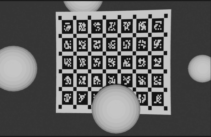
Consider the below video. In the scene, there’s a calibration board tilted away from the camera and a few equally-sized spheres placed around it. As the video progresses, the focal length sweeps from wide to narrow. Simultaneously, the camera moves backwards to approximately maintain the size of the board in the image.

However, nothing in this scene is actually moving. This process is called a dolly zoom. As the focal length narrows, the scene appears to compress. Even though the closest and furthest spheres are twelve meters apart, they appear similarly sized. Also, the far edge of the board tilted away from the camera appears to pull in, with the board's apparent shape under projection going from a trapezoid to a rectangle.

Foreshortening is very important to observing focal length; we’ll see why in a bit.

How does calibration work?

First, we’ve got to take a brief detour to discuss how calibration works. We’ve got a series of blog posts about this if you want more detail, but we’ll do a short overview here.

In a typical calibration scenario, we take images of a target of known dimensions. The target has detectable and uniquely-identifiable features which correspond to 3D feature locations in some model coordinate system. We project the 3D features into the image using the current estimate of the camera intrinsics and find the error between the projected values and the detections. This is called reprojection error. The calibration process is an optimization problem whose objective is: “adjust the intrinsics in order to minimize (the sum-squared of) reprojection error”.

In order to project a 3D point into the image, the 3D point has to be in the camera’s coordinate system. The 3D points described by the target’s design are in some relatively-arbitrary model coordinate system. In order for calibration to work, we also have to jointly estimate the camera-from-model transform for each image. That per-image transform is a nuisance parameter: something we have to estimate but isn’t actually of interest to us in the end.

The reason for bringing up details of the calibration algorithm is that it highlights a natural ambiguity that arises when calibration data isn’t captured correctly. When a planar target’s normal is aligned with the camera optical axis, focal length can freely trade off with the Z component (or depth distance) of the camera-from-model transform. Which means that in minimizing reprojection error you can choose any focal length and the camera-from-model depth (i.e. Z component) will simply compensate and vice versa. In this scenario, it is impossible to learn the focal length.

This is why we suggest users capture a wide variety of angles between the board normal and the camera’s axis. When the board is tilted away from the camera, focal length becomes observable through the foreshortening effects (like we saw in the previous video), because the board by virtue of being tilted exists at a variety of depths relative to the camera.

The following video highlights the aforementioned ambiguity. The scene is the same as above, except the board’s normal is aligned to the camera’s optical axis. As before, the camera’s field of view gets gradually narrower as the camera moves backwards. Again— nothing else is moving. In this scenario, it’s possible to exactly preserve the appearance of the board in the image even as the camera’s position and focal length change wildly.

It’s important to highlight that this isn’t a binary thing. Calibration doesn’t just all of a sudden work as soon as you go one degree off the optical axis. All sorts of inaccuracies introduce error into the process and reduce the observability of the focal length and thus your margin for error in the calibration data capture process. These include:

• static inaccuracy of the board

• frame-to-frame non-rigid warping of the board

• blur (both motion and defocus)

• resolution (both sensor and lens sharpness/spatial resolution)

• sensor noise and compression artifacts

• detector algorithm limitations

Back to Focal Length

So fine, you say, I’ll tilt the board and git gud at angles or whatever. What does this have to do with NFOV cameras? The problem is that NFOV cameras have very little foreshortening effect no matter how much you tilt them.

Here’s the last frame (i.e. at the most narrow FOV) of the first video. That board is tilted 35 degrees off-axis, but you wouldn’t guess that from the image. The far side (left) of the board is about the same size as the near side (right) of the board. There probably is some perspective effect here which, in a totally-ideal, noise-free case, might be enough, but practically when calibrating with images like this, depth and focal length are going to tradeoff massively.

For marginal cases, there are some simple ways to address this. You can tilt the board or camera more if you haven’t already. Often it’s straightforward to tilt the board, but “tilting” the camera with an extremely narrow focal length while keeping the target in view requires moving the camera over a very large area, which might be logistically impractical. Conversely, tilting the board too much will eventually cause feature detectors to fail— 45° off axis is a good rule of thumb.

You could also make a larger board, which when tilted will cover a greater range of depths, helping the observability of foreshortening and thus focal length. This too has limitations as the size of the board will have major impact on cost, availability, accuracy, rigidity, ease-of-manipulation, and space requirements.

Failing these two simple fixes, the next step is to think beyond just planar targets.

3D Targets (probably) aren’t enough

A solution one might naturally consider would be to build a target that innately has some variation in depth, i.e. one that’s not a board or plane. The calibration process does not fundamentally require a planar target: the camera-from-model transform can be estimated with an algorithm like PnP provided you have a reasonable guess for intrinsics.

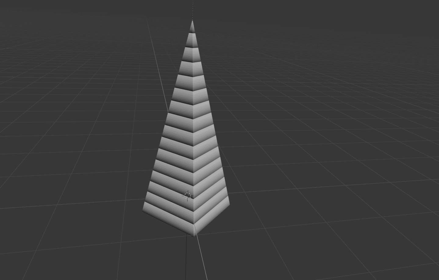
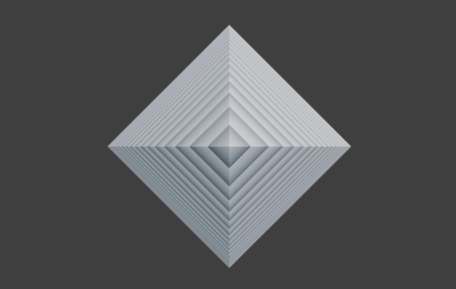
A non-planar target is a target that has variation in all spatial dimensions, and thus will hopefully display some foreshortening when imaged, no matter what its orientation relative to the camera is. As an example, consider a pyramid shaped object, with its apex pointed at the camera, and some features on its faces. We can see foreshortening in the spacing of the lines when imaged, and we can do so without having to tilt the object away from the camera.

Non-planar targets certainly represent an interesting approach to calibration, and they have their niche uses. However, a lot of the same drawbacks you’d get from building a large board and tilting it still apply. The target still needs to be large (think like several meters long) to get the desired effect, it's sensitive to initial conditions, and it is substantially harder to build and come up with a reliable detection algorithm.

In contract, planar targets are advantageous for a few reasons:

• They’re relatively easy to describe with just a few parameters (e.g. width, height, spacing)

• They’re easily made (just print them)

• The planar arrangement imposes some invariants that make writing detectors easier. For example, a planar circle is an ellipse under projection. Grids of features will have some understandable relation under projection, which may make decoding targets easier.

• The camera-from-model transform can be more-easily bootstrapped by estimating a planar homography.

The MetriCal Approach

To provide a (patent-pending!) user-friendly approach to narrow field of view camera calibration, we’ve combined the advantages of planar and non-planar targets by using multiple planar targets merged together. Instead of relying on the size and relative angle of a single board to observe foreshortening and thus focal length, we’ll use multiple boards offset at different depths from the camera. Since the calibration target consists of multiple boards, we get the advantages of board targets (easy construction, well-known detector algorithms etc.), and we get to build a composite target with a large depth range simply by spacing the boards apart.

In this video, two boards are set a few meters apart along the camera’s optical axis. We set up a similar dolly-zoom to preserve the appearance of the left board. Notice how the right board appears to grow as the focal length gets narrow. This shows how we cannot trade-off a single camera-depth value and focal length to preserve the appearance of two objects at different depths.

It does not, however, suffice to simply use multiple boards. In a typical calibration scenario, the camera-from-board transform has to be estimated for every board in each image. Estimating that transform is where the focal length ambiguity rears its head, and having two boards with two camera-from-board transforms per image is really no different. The trick is to merge the board targets into one calibration target so that only one transform per image need be estimated. Since the individual targets are at different depths, no single camera-from-board depth value can trade off with focal length in the optimization. This means focal length has become unambiguous.

In order to merge the board targets together such that a single camera-from-target transform is sufficient, we have to know the spatial relationship between the boards. The simplest way to learn those relationships is to survey the board-system with a calibrated camera. Fortunately, this is something that MetriCal can already do today so long as you have at least one non-NFOV camera!

So for narrow-field-of-view cameras, calibration becomes a multi-step process and requires an auxiliary camera. Many modern perception sensor suites contain multiple cameras of different focal lengths. Those cameras need to be calibrated regardless, so often this requirement is no real imposition.

The process generally looks like this:

1. A target field with targets at varying depths is constructed.

2. Data is captured with a more easily calibrated camera (i.e. a wider FOV one). If the target field and camera are amenable to it, one dataset can be used to jointly calibrate this camera and survey the target field in one pass. If not, separate calibration and survey datasets are captured.

3. The camera is calibrated and the target field is surveyed with MetriCal either in one pass or separately. This is done via MetriCal’s calibrate step.

4. The target field survey and calibration are used to create a consolidated object space configuration for the target field. This is done via MetriCal’s consolidate-object-spaces step.

5. Data is captured with the narrow field of view camera. The camera should observe the target field as it was surveyed. Generally the same sorts of data capture requirements apply as always. The image space should be well-covered.

6. The narrow field of view dataset and consolidated object space configuration are used to calibrate the narrow field of view camera.

Try It Out!

At the time of writing, we’ve just released version 15.0.0 of MetriCal. This version focused hard on quick start time for new MetriCal users, as well as improvements for production line setups. Some customers are already using the technique above in their production line!

If you want to try it out yourself, follow our Calibration Guides in the MetriCal documentation. There, you can find demo datasets that show off what MetriCal can do, along with a ton of other tips and tricks for multi-modal calibration.